Engineering Game Types

Introduction

Let’s suppose we want to change a game’s type to increase (or decrease) alignment¹, or otherwise engineer the game to have desired characteristics (similar to social choice). If we assume the game payoffs are functions of the parameters of each player, we can determine what interventions on the parameters map to which game types (or vice-versa).

In the invariant coordinates post, we developed ways of describing games independently of the names attached to their strategies. We used computational invariant theory to construct polynomial functions of the payoffs that remain unchanged when strategies are relabeled. A sufficiently rich collection of these invariants distinguishes games up to relabeling and lets us describe game classes through equations and inequalities. What’s more, we can theoretically use different groups to obtain coarser/finer quotients. For example, we could identify player permutations when player identity is irrelevant, or remove additive payoff baselines when only incentive differences matter. The choice determines which differences between games the description retains.

In Games, Invariants, and Alignment, I explored how to read these coordinates. We can organize a game’s payoffs by who receives them, or by the individual, pairwise, and higher-order interactions that produce them. Within each interaction component, quadratic invariants measure the strength of that component’s effects and how different players’ payoffs vary together or in opposition. Higher-degree invariants capture additional structure within or between the components. This gives us a way to locate alignment and conflict within a game, and to move between the individual and group perspectives while retaining the underlying payoff information.

These descriptions let us return to a question raised in Differentiable Game Canonicalization: when does Stag Hunt turn into Chicken? In Differential Games and Stag Hunt, I constructed a pursuit-evasion model, extracted a normal-form payoff table from the model’s strategy profiles, and proposed connecting such a table to game classification. Connecting such models to invariant descriptions lets us ask which parameter changes produce desired game properties, which preserve them, and when the available controls make a target impossible.

Let \(\theta \in \Theta\) collect the players’ parameters. These determine the payoffs \(u(\theta)\) and therefore an invariant description \(z(\theta)\):

\[ \theta \longmapsto u(\theta) \longmapsto z(\theta) \]

Here \(z(\theta) = I(u(\theta))\). To obtain the desired game type output, we seek parameters where the invariant description lies in the target region:

\[ z(\theta) \in \mathcal{Z}_{\mathrm{target}} \]

For instance, if \(z_j\) measures “alignment” in a particular interaction, we can require \(z_j \ge \tau\) for some chosen threshold \(\tau\). Starting from \(\theta_0\), we let \(v\) specify an intervention and let \(\psi\) describe how the intervention changes the parameters:

\[ \theta' = \psi(\theta_0, v) \]

The map \(\psi\) can be nonlinear and can couple different parameters (it could be a neural network, for instance, or some other function of the parameters, ideally differentiable to run some of the later functionality but it is not a necessity).

Let \(\mathcal{C}(\theta_0)\) contain the permitted interventions, including permissions, bounds, and any budget, with resulting parameters in \(\Theta\). Working backward gives the interventions that meet the target:

\[ \mathcal{F}(\theta_0) = \{v \in \mathcal{C}(\theta_0) : z(\psi(\theta_0, v)) \in \mathcal{Z}_{\mathrm{target}}\} \]

Thus, every member of \(\mathcal{F}(\theta_0)\) is a successful intervention. A proof that this set is empty certifies that the available controls can’t achieve the target. If we also specify an intervention cost \(c\), we can ask for a least-cost member if such a minimum exists:

\[ v^* \in \underset{v \in \mathcal{F}(\theta_0)}{\operatorname{argmin}} c(v) \]

The resulting game is

\[ u^* = u(\psi(\theta_0, v^*)) \]

In this post, I build code for describing and controlling game types, then use a series of examples to explore which interventions succeed and what we can prove about them.

Mathematical Preliminaries

We start with a supplied model, which includes

1. a collection of players and their actions
2. parameters describing the players and how they take actions
3. a rule that maps joint choices and parameter values to outcomes and payoffs (the game)
4. the permitted interventions
5. the property or properties we want to achieve

Fixing the parameters gives one game, while varying the parameters gives an entire family of games.

We choose the transformations under which two descriptions count as the same game the same way we did in previous posts.² Here these are independent relabelings of each player’s actions, as in the earlier post. This choice determines the invariant ring, which is the polynomial functions of payoffs unchanged by those relabelings.

Let individual \(i\) have \(m_i\) actions. Write \(A = \prod_i A_i\) for the joint action space and \(N = \prod_i m_i\) for the number of joint actions. A game is a payoff tensor

\[ u \in V = \mathbb{R}^{n \times m_1 \times \cdots \times m_n} \]

The entry \(u_p(a)\) is individual \(p\)’s payoff at joint action \(a\). Individuals may have different numbers of actions.

A payoff model assigns a tensor \(u(\theta)\) to each allowed parameter choice \(\theta \in \Theta\). An intervention \(v\) changes those parameters through the supplied map \(\psi\). Composing the two maps gives

\[ v \longmapsto \psi(\theta_0, v) \longmapsto u(\psi(\theta_0, v)) \]

Applying invariant measurements to the resulting payoffs describes how the intervention changes the game. Desired properties become conditions on those measurements or on payoff differences that express the required incentives. Substituting the composed map turns those conditions into constraints on the permitted interventions.

The following section gives a series of vignettes that use these objects to analyze and control games and manipulate game types. The appendix begins with the shared implementation, followed by the derivations and code for the operations used in each example.

Vignettes

In this section, we’ll use algebraic descriptions of games to guide interventions that change the game type. In each vignette, we’ll start with a game, apply a supplied intervention, and then inspect the resulting output game. The examples also show how to find successful interventions, check a route, maintain desired game properties as conditions change, and determine whether the available controls are sufficient. Subsequent examples change the available controls, the number of individuals and actions, or the model generating the payoffs.

Every example uses the same compositional setup from the preliminaries. Write \(u_v\) for the game produced by intervention \(v\) and \(z_v\) for the resulting invariant measurements:

\[ \begin{aligned} u_v &= u(\psi(\theta_0, v))\\ z_v &= I(u_v) \end{aligned} \]

In code, family maps parameters to games, parameters maps interventions to parameters, and controlled_games = parameters.then_apply(family). A Control bundles the parameter map with permissions, bounds, and cost. When we specify a target region \(\mathcal{T}\), design(family, control, target) adds the condition \(u_v\in\mathcal{T}\) and retains the resulting feasible region \(\mathcal{F}\) (see the Appendix for more information about the code).

The figures depicting each vignette use selected invariant measurements of these same payoff tensors. Each point represents a game, and each surface or curve represents a supplied family.

1. Applying an Intervention and Changing a Game Type

Figure 1: Consider a supplied intervention in each of two games. On the left, an update changes a two-individual game’s joint payoff effects from opposed to aligned. On the right, an update changes how a three-way term contributes to the payoffs of three individuals with different action counts. Both calculations evaluate the payoff tensor, apply invariant measurements, and check the green target.

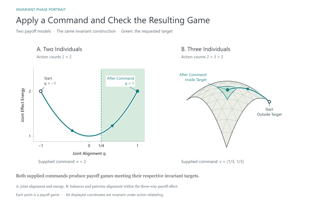
Suppose we have a parameterized game and a desired game type, expressed as a region in invariant coordinates. Given a proposed parameter update, we want to compute the resulting game and check whether the update produces the desired type.

Problem. Given a payoff model, starting parameters, an invariant target, and a supplied intervention, does the resulting game belong to the desired type?

Procedure.

1. Apply the parameter map \(\psi\) to the input command \(v\) to obtain the updated parameters.

2. Evaluate the payoff model at those parameters to obtain the payoff tensor \(u_v\).

3. Apply the invariant map \(I\) to that tensor to obtain \(z_v\).

4. The intervention succeeds when the command is permitted and the resulting invariant vector belongs to the desired region

   \[ z_v\in\mathcal Z_{\mathrm{target}} \]

5. Evaluating the same invariant map on the starting game shows what changed.

The starting parameters are bound into \(\psi\).

Code. We supply the following objects:

Code Object	What the Object Supplies
family	A Map from model parameters to a Game containing the payoff tensor and action counts.
control	A Control containing the command-to-parameter map, the permitted command region, and the intervention cost.
measurements	A Map from a Game to the selected invariant values.
desired_type	A Region of invariant values satisfying the requested equations or inequalities.
theta0	The starting parameter vector.
command	The supplied intervention vector.

The composition makes the construction explicit:

controlled_games = control.parameters.then_apply(family)
controlled_types = controlled_games.then_apply(measurements)
successful_commands = control.allowed & desired_type.pullback(controlled_types)

starting_game = family(theta0)
resulting_game = controlled_games(command)
starting_measurements = measurements(starting_game)
resulting_measurements = controlled_types(command)
intervention_valid = successful_commands.contains(command)

pullback substitutes the composed map into the target conditions. The resulting region contains every permitted command whose payoff tensor has the desired invariant values. The appendix implements this substitution.

Example: Turning Opposed Payoffs into Aligned Payoffs

Consider two individuals choosing binary settings, written as \(x\) and \(y\). A shared score \(xy\) depends on both choices. The first individual’s payoff is the score, while a configurable weight \(\theta\) determines how the score contributes to the second individual’s payoff

\[ u_0(x,y)=xy \qquad u_1(x,y)=\theta xy \qquad x\in\{-1,1\} \quad y\in\{-1,1\} \]

A negative weight makes the two payoffs move in opposite directions. A positive weight makes the payoffs move together. We want the latter property with a specified minimum strength, expressed using the joint alignment coordinate from Games, Invariants, and Alignment

\[ q(u)=M_{\{0,1\}}[0,1] \qquad \mathcal Z_{\mathrm{target}}=\{q:q\ge\tau\} \qquad \tau>0 \]

The entry \(M_S[p,q]\) is the uniformly averaged product of the interaction effects on recipients \(p\) and \(q\). These measurements are unchanged by independent action relabelings. The target specifies positive alignment in this interaction. A finer game type would require additional invariant conditions.

Instance. Start at \(\theta_0=-1\), set \(\tau=1/4\), and permit commands \(0\le v\le2\). Supply the command \(v=2\) and parameter map \(\psi(v)=\theta_0+v\). The additive update belongs to this example’s model. The composition also accepts nonlinear parameter maps.

Supply the Payoff Tensor Model and Target

The arrays x and y evaluate the action values at all four joint choices. binary_base has shape (2, 2, 2), with the recipient on the first axis. The coefficient tensor changes only the second individual’s payoffs. polynomial evaluates the supplied coefficient tensors at a parameter vector.

def add_payoff_terms(changes, payoffs, theta):
    return payoffs + changes(theta)


x, y = np.meshgrid(exact([-1, 1]), exact([-1, 1]), indexing="ij")
joint_score = x * y
zero_table = exact(np.zeros((2, 2), dtype=int))
binary_base = np.stack([joint_score, zero_table])
binary_coefficient = np.stack([zero_table, joint_score])
binary_changes = polynomial([((1,), binary_coefficient)])
binary_family = Game(binary_base, (2, 2)).with_payoff_rule(
    partial(add_payoff_terms, binary_changes)
)

binary_start = exact([-1])
binary_parameters = Map(lambda v: like(binary_start, v) + v)
binary_allowed = ge(Map(lambda v: v), 0) & ge(Map(lambda v: 2 - v), 0)
binary_control = Control(
    binary_parameters, binary_allowed, Map(lambda v: v.sum(axis=-1)),
    ("joint_weight_change",),
)
binary_measurements = gram((0, 1), 0, 1)
binary_desired_type = ge(Map(lambda q: q), sp.Rational(1, 4))
binary_command = exact([2])

The application supplies payoffs, controls, and a target. gram supplies the invariant measurement from the shared library. No formula for the invariant as a function of the command has been supplied.

Solving the Example. Pass these objects through the composition above:

binary_games = binary_control.parameters.then_apply(binary_family)
binary_types = binary_games.then_apply(binary_measurements)
binary_successful = binary_allowed & binary_desired_type.pullback(binary_types)
binary_before = binary_family(binary_start)
binary_after = binary_games(binary_command)
binary_before_measurement = binary_measurements(binary_before)
binary_after_measurement = binary_types(binary_command)
binary_intervention_valid = binary_successful.contains(binary_command)

Result. The invariant changes from \(q=-1\) to \(q=1\). The resulting game belongs to the desired region because \(1\ge1/4\), and the command satisfies the bounds. The returned objects include the new payoff tensor and the successful target check.

Read and Differentiate the Composed Map

Symbolic evaluation of the tensor model and Gram contraction gives

\[ q(u(\psi(v)))=-1+v \]

The same computation accepts Torch values and differentiates through the payoff tensor and invariant measurement:

binary_command_symbol = sp.symbols("v", real=True)
binary_symbolic_type = binary_types(exact([binary_command_symbol]))
binary_sensitivity = torch.func.jacfwd(binary_types)(
    torch.tensor([0.0], dtype=torch.float64)
)

The derivative is \(1\). Relabeling either individual’s actions leaves the measured value unchanged.

The same forward calculation also applies to more individuals and unequal action counts. We now supply a three-individual model that will serve as the running example for the control questions that follow.

Example: Changing a Three-Individual Game

Now consider three individuals with separate action sets. Each payoff combines a local term, terms depending on pairs of choices, and a term depending jointly on all three choices. Such a model can describe individual rewards in a system where a joint outcome depends on several decisions. We can configure how strongly each payoff responds to that joint outcome.

Write \(Y_S\) for the term depending on the choices of individuals in \(S\), and \(\gamma_i\) for the weight of the three-way term in individual \(i\)’s payoff. We hold the combined three-way contribution fixed by requiring \(\sum_i\gamma_i=1\). Initially only the first payoff contains that contribution. We want every individual’s payoff to have a specified minimum alignment with the combined three-way effect.

Use the same Gram construction as in the binary case, now for \(S=\{0,1,2\}\). The matrix has one row and column per payoff recipient. Summing row \(i\) measures alignment between that recipient’s effect and the combined effect

\[ z_i(u)=\sum_{q=0}^2M_{\{0,1,2\}}[i,q] \qquad \mathcal Z_{\mathrm{target}}=\{z:z_i\ge\tau\ \text{for every }i\} \]

These row sums are polynomial invariants formed from the same gram measurements. The desired type concerns the three-way interaction. Pairwise and individual effects remain in the payoff tensor, even though this particular target places no requirements on those components.

Instance. Give the individuals action values \(\{0,1\}\), \(\{0,1,2\}\), and \(\{0,2\}\). A joint choice supplies \((x_0,x_1,x_2)\) to the payoff function. The local term for recipient \(i\) is \(-x_i^2/4\). Pair terms are \(Y_{\{i,j\}}=x_ix_j\), and the three-way term is \(Y_{\{0,1,2\}}=x_0x_1x_2\). Evaluating the twelve joint choices produces a payoff tensor with shape (3, 2, 3, 2).

For each pair \(i<j\), the pair term has weight \(\alpha_{ij}\) in recipient \(i\)’s payoff and \(1-\alpha_{ij}\) in recipient \(j\)’s payoff. The independent parameters are

\[ \theta=(\alpha_{01},\alpha_{02},\alpha_{12},\gamma_0,\gamma_1) \qquad \gamma_2=1-\gamma_0-\gamma_1 \]

For the supplied intervention, use \(v=(1/3,1/3)\). Start with pair weights \(1/2\) and three-way weights \((1,0,0)\). The permitted command \(v=(v_1,v_2)\) changes the three-way weights to \((1-v_1-v_2,v_1,v_2)\) and leaves the pair weights fixed. Require nonnegative commands with \(v_1+v_2\le1\), record cost \(v_1+v_2\), and choose \(\tau=1/24\). This command changes the three-way weights to \((1/3,1/3,1/3)\). We evaluate the resulting game and test the invariant target.

Supply the Three-Individual Payoff Model and Target

project_base and the five coefficient tensors encode the payoff formula. The same polynomial evaluator used in the binary example combines these tensors with parameter values. project_parameters supplies the parameter update. project_measurements collects the three invariant row sums, and project_desired_type requires every value to meet the bound.

project_shape = (2, 3, 2)
effort_menus = (exact([0, 1]), exact([0, 1, 2]), exact([0, 2]))
efforts = np.meshgrid(*effort_menus, indexing="ij")
project_costs = np.stack(efforts) ** 2 * sp.Rational(1, 4)
project_base = -project_costs
project_coefficients = []

for i, j in combinations(range(3), 2):
    output = efforts[i] * efforts[j]
    project_base[j] += output
    transfer = exact(np.zeros((3,) + project_shape, dtype=int))
    transfer[i], transfer[j] = output, -output
    project_coefficients.append(transfer)

joint_output = np.prod(efforts, axis=0)
project_base[2] += joint_output
for i in (0, 1):
    transfer = exact(np.zeros((3,) + project_shape, dtype=int))
    transfer[i], transfer[2] = joint_output, -joint_output
    project_coefficients.append(transfer)

project_terms = [
    (tuple(int(i == j) for j in range(5)), coefficient)
    for i, coefficient in enumerate(project_coefficients)
]
project_changes = polynomial(project_terms)
project_family = Game(project_base, project_shape).with_payoff_rule(
    partial(add_payoff_terms, project_changes)
)

project_start = exact([sp.Rational(1, 2)] * 3 + [1, 0])
project_actuator = exact([[0, 0], [0, 0], [0, 0], [-1, -1], [1, 0]])
project_parameters = Map(
    lambda command: like(project_start, command)
    + command @ like(project_actuator, command).T
)
project_command = exact([sp.Rational(1, 3), sp.Rational(1, 3)])

joint_grams = tuple(
    tuple(gram((0, 1, 2), i, j) for j in range(3))
    for i in range(3)
)
joint_alignment = Map(lambda game: stack([
    sum(entry(game) for entry in row) for row in joint_grams
], axis=-1))
collective_joint_energy = Map(lambda game: joint_alignment(game).sum(axis=-1))
project_measurements = joint_alignment
project_threshold = sp.Rational(1, 24)
project_desired_type = ge(Map(lambda z: z), project_threshold)
project_target = project_desired_type.pullback(project_measurements)
project_allowed = (
    ge(Map(lambda v: v), 0)
    & ge(Map(lambda v: 1 - v.sum(axis=-1)), 0)
)
project_control = Control(
    project_parameters,
    project_allowed,
    Map(lambda v: v.sum(axis=-1)),
    ("weight_to_second", "weight_to_third"),
)

Solving the Example. Use the same composition and target check as in the two-individual case:

project_games = project_control.parameters.then_apply(project_family)
project_types = project_games.then_apply(project_measurements)
project_successful = (
    project_allowed & project_desired_type.pullback(project_types)
)
project_before = project_family(project_start)
project_after = project_games(project_command)
before_measurements = project_measurements(project_before)
after_measurements = project_types(project_command)
project_initially_in_target = project_target.contains(project_before)
project_target_reached = project_target.contains(project_after)
project_intervention_valid = project_successful.contains(project_command)

Result. The supplied command changes the invariant vector from \((1/6,0,0)\) to \((1/18,1/18,1/18)\). The starting game fails the target because two coordinates fall below \(1/24\). The resulting game meets every bound, and the command is permitted.

The payoff tensor now has shape (3, 2, 3, 2). The three-way effect is nonzero, and the middle individual’s three actions each matter. The same invariant contractions and region operations handle both examples. We will use this three-individual model for the inverse-design, maintenance, and control-authority questions below.

Differentiate and Check the Three-Individual Example

The composed map also carries Torch derivatives through the larger payoff tensor:

numerical_project_command = torch.tensor([.2, .1], dtype=torch.float64)
project_sensitivity = torch.func.jacfwd(project_types)(numerical_project_command)

Checks compare Torch and symbolic derivatives, verify invariance under all 24 independent action relabelings, and check total payoff preservation at every joint choice. In the resulting game, each of the middle individual’s three actions is uniquely best against some choices of the other two.

The command was supplied in both examples. We next keep the three-individual model and target, and ask the framework to find a successful command.

2. Inverse Design: Feasible Regions and Minimum-Cost Interventions

Figure 2: Consider three individuals whose payoffs combine individual, pairwise, and three-way terms. We can change the weights assigning the three-way term to each payoff. The green region contains games meeting a minimum alignment with the combined effect for every individual. Budget curves show which games the permitted updates can reach. The first successful budget changes two weights by one quarter each.

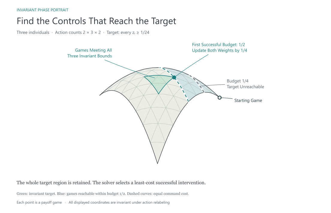
Suppose we have specified the desired invariant type and know which parameters we can change. We now want to find interventions that produce that type and compare the costs of the successful choices.

Problem. Given a payoff model, an invariant target, and permitted controls, return the successful command region and a least-cost member when a minimum exists.

Procedure.

1. Compose the parameter update, payoff model, and invariant measurements as before.

2. Pull the desired region back through that composition and intersect with the permitted controls.

3. Leave the command unspecified and ask a solver to choose from the resulting region

   \[ \mathcal F=\{v\in\mathcal C:I(u_v)\in\mathcal Z_{\mathrm{target}}\} \]

When the composed constraints and cost are affine, solve_affine returns an optimum or an infeasibility certificate. Other expressions need a suitable solver.³ The payoff and invariant maps defining the question remain the same.

Code. family, control, measurements, and desired_type have the meanings given above. command_symbols supplies one real symbol per command coordinate. The corresponding target on games is the pullback of the desired invariant region:

target = desired_type.pullback(measurements)
problem = design(family, control, target)
answer = solve_affine(problem, command_symbols)

design packages the composed game map, successful command region, and cost. problem.feasible is the same region constructed explicitly in the first vignette. The solver receives that region and derives constraints by evaluating the supplied maps symbolically.

Example: Finding a Command for the Three-Individual Game

Return to the three-individual model from the first vignette. Keep the payoff model, starting parameters, invariant target, control bounds, and cost. The previous command assigned equal weights to the three-way term. We now ask which commands meet the target and which successful choice costs least.

Instance. The initial three-way weights are \((1,0,0)\). A permitted command has \(v_1\ge0\), \(v_2\ge0\), and \(v_1+v_2\le1\), and produces weights \((1-v_1-v_2,v_1,v_2)\). Retain the target \(z_i\ge1/24\) for every individual and cost \(v_1+v_2\).

Solving the Example. Package the existing maps and target with design, then pass the unknown command coordinates to the solver:

project_problem = design(project_family, project_control, project_target)
project_command_symbols = sp.symbols("v1 v2", real=True)
project_answer = solve_affine(project_problem, project_command_symbols)
project_solution = project_problem.select(exact(project_answer.data["point"]))
project_solution_valid = project_answer.verify() and project_solution.verify()

The solver obtains the expressions below by evaluating the payoff tensor and invariant map at symbolic command values

\[ z(u_v)=\frac16\begin{pmatrix}1-v_1-v_2\\v_1\\v_2\end{pmatrix} \]

Substitution into the invariant target gives the successful command region

\[ \mathcal F=\left\{v:v_1\ge\frac14\quad v_2\ge\frac14\quad v_1+v_2\le\frac34\right\} \]

The Gram measurements are quadratic in arbitrary payoff tensors. On this family, the combined three-way effect stays fixed, so these row sums become affine functions of the commands. The affine solver therefore applies to the composed invariant conditions.

Result. The returned command is \((1/4,1/4)\), with minimum cost \(1/2\). The resulting three-way weights are \((1/2,1/4,1/4)\) and the invariant vector is \((1/12,1/24,1/24)\). Every successful command costs at least \(1/2\). Adding a smaller budget yields a checked infeasibility certificate.

The supplied command \((1/3,1/3)\) from the first vignette also succeeds, at cost \(2/3\). The computed command meets the same invariant target at lower cost.

Check the Returned Region and Certificate

project_problem.feasible retains every successful command. Reusing the original command checks that the forward calculation and the solver use the same region:

project_intervention = project_problem.select(project_command)
project_intervention_valid = project_intervention.verify()

Exact checks compare this region with project_successful from the first vignette. The optimality certificate verifies the lower bound on cost, and direct evaluation checks the returned game’s invariant values. Changing the target threshold changes the computed optimum through the same calls.

3. Constrained Reachability: Safe Paths and Obstructions

Figure 3: Consider a system whose parameters must change gradually. Both routes end at the same desired three-individual game, but changing the controls together crosses a forbidden region. Changing the third individual’s weight first gives a verified safe route. The surface uses the same invariant coordinates as the opening example.

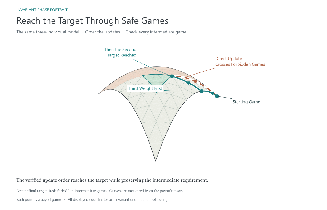
Suppose we know a successful intervention, but applying the whole command at once is unavailable. A sequence of updates must preserve an additional requirement while changing the game. Reaching an acceptable endpoint and reaching that endpoint safely are different questions.

Problem. Find a path of permitted commands from the current game to the invariant target while remaining in a supplied safe region.

Procedure.

1. Pull the safe game region back through the same command-to-game map. This gives the commands that produce safe games.
2. Generate candidate paths in command space and check every segment against that region.
3. Check that the final command also satisfies the original target.

A verified route establishes safe reachability. Failure of the candidate search alone establishes no obstruction.

Code. problem is the composed control problem, safe_games is a region of payoff tensors, and start and goal are command vectors. The procedure below searches the orders in which individual controls can change. segment_ok substitutes each proposed segment into the constraints and checks the whole parameter interval.

safe_commands = control.allowed & safe_games.pullback(problem.games)
route = find_axis_route(safe_commands, start, goal)
endpoint_valid = route is not None and problem.feasible.contains(route[-1])

Example: Ordering Updates in the Three-Individual Game

Return to the same payoff model and target from the previous example. Suppose a staged update requires the second individual’s joint response to stay small until the third individual’s response has reached the target threshold. Express that requirement directly in the measured invariant values

\[ \mathcal S=\left\{u:z_1(u)\le\frac1{48}\right\} \cup \left\{u:z_2(u)\ge\frac1{24}\right\} \]

We start at command \((0,0)\) and want to reach the computed command \((1/4,1/4)\). The model, controls, measurements, and final target are unchanged. Only the requirement on the intermediate games is new.

Construct and Check the Routes

project_safe_games = (
    ge(Map(lambda game: -project_measurements(game)[..., 1]), -sp.Rational(1, 48))
    | ge(Map(lambda game: project_measurements(game)[..., 2]), sp.Rational(1, 24))
)
project_safe_commands = project_allowed & project_safe_games.pullback(project_games)
route_start = exact([0, 0])
route_goal = project_solution.command
project_route = find_axis_route(project_safe_commands, route_start, route_goal)
project_direct_safe = segment_ok(project_safe_commands, route_start, route_goal)
project_route_valid = project_route is not None and project_target.contains(project_games(project_route[-1]))
matched_changes = Map(lambda t: stack([t[..., 0], t[..., 0]], axis=-1))
path_parameter = sp.Symbol("t", real=True)
matched_safe_set = univariate_region(
    project_safe_commands.pullback(matched_changes), path_parameter, sp.Interval(0, sp.Rational(1, 2))
)
matched_target_set = univariate_region(
    project_successful.pullback(matched_changes), path_parameter, sp.Interval(0, sp.Rational(1, 2))
)

Solution. The procedure returns

\[ (0,0)\longrightarrow(0,1/4)\longrightarrow(1/4,1/4) \]

The first segment keeps \(z_1=0\) while increasing \(z_2\). The second segment increases \(z_1\) after \(z_2\) has reached \(1/24\). Both complete segments pass the exact checks. The direct segment fails because the second individual’s response grows too early.

There is also a simple impossibility certificate. Suppose the actuator forces the two changes to match, so commands have the form \((t,t)\). Pulling the safe region and target back along that actuator gives

\[ \mathcal S_t=[0,1/8]\cup[1/4,1/2] \qquad \mathcal F_t=[1/4,3/8] \]

The initial value lies in the first connected component of the safe set, while every target value lies in the second. No continuous safe path through this restricted actuator reaches the target. The obstruction follows from the computed regions and continuity, rather than a failed path search.

4. Robust Control: Maintaining a Desired Game Type

Figure 4: Consider a game whose parameters drift while a controller tracks a preferred invariant value. The invariant-space panel shows how the command filter preserves the target. The time-series panels compare PID with physical actuator limits against PID using the invariant constraint filter, then show which command proposals the filter changes. All measurements come from the same three-individual payoff model.

A successful intervention may not remain successful when the environment changes. Suppose we observe the current parameters, choose an adjustment, and then an unknown disturbance changes the parameters again. We want a rule for choosing adjustments that keeps the game in the desired region.

Problem. Determine which commands preserve the invariant target for every allowed disturbance, then choose a low-cost command from that region.

Procedure.

1. Compose the supplied state update with the payoff model and invariant target.
2. Require the resulting game to satisfy the target for every disturbance. When the target is convex in the updated state and the update depends affinely on a disturbance box, checking every box vertex is sufficient.
3. Retain the resulting relation, which specifies the successful commands at each observed state.
4. Solve the corresponding control problem whenever a new state is observed.

Code. state_target is the invariant target pulled back to model parameters. transition maps a state-command vector and disturbance to the next parameter vector. disturbance_bounds contains the lower and upper bound of each disturbance coordinate.

robust_commands = box_preimage(state_target, transition, disturbance_bounds)

The returned Region retains the constraints on both current states and commands. The vertex construction requires the convexity and affine-dependence assumptions above. For polynomial nonlinear disturbances, use solve_polynomial on the original problem with the disturbance symbols and bounds.

Example: Correcting Drift in the Same Game Family

Suppose the two adjustable joint weights must remain equal. Write the three weights as \((1-2t,t,t)\). Substituting this parameterization into the same invariant target gives

\[ \frac14\le t\le\frac38 \]

An adjustment \(v\) precedes a disturbance \(w\). The supplied update and bounds are

\[ t'=t+v+w \qquad |v|\le\frac1{24} \qquad |w|\le\frac1{48} \]

Construct the Robust Region and Solve for Feedback

shared_project_parameters = Map(lambda t:
    like(project_start, t)
    + t[..., :1] * like([0, 0, 0, -2, 1], t))
shared_project_games = shared_project_parameters.then_apply(project_family)
shared_target = project_target.pullback(shared_project_games)
drift_symbol = sp.Symbol("t", real=True)
drift_interval = univariate_region(shared_target, drift_symbol, sp.Interval(0, sp.Rational(1, 2)))
drift_radius = sp.Rational(1, 48)
drift_limit = sp.Rational(1, 24)


def drift_transition(state_command, disturbance):
    return stack([state_command[..., 0] + state_command[..., 1] + disturbance[..., 0]], axis=-1)


robust_moves = box_preimage(shared_target, drift_transition, ((-drift_radius, drift_radius),))
robust_moves = robust_moves & ge(Map(lambda tv: tv[..., 1]), -drift_limit)
robust_moves = robust_moves & ge(Map(lambda tv: -tv[..., 1]), -drift_limit)


def drift_pair(current, command):
    return stack([like(current, command) + command[..., 0] * 0, command[..., 0]], axis=-1)


def adjusted_parameter(current, command):
    return stack([like(current, command) + command[..., 0]], axis=-1)


absolute_above_positive = Map(lambda vc: vc[..., 1] - vc[..., 0])
absolute_above_negative = Map(lambda vc: vc[..., 1] + vc[..., 0])
absolute_cost = Map(lambda vc: vc[..., 1:].sum(axis=-1))


def drift_problem(current):
    parameters = Map(partial(adjusted_parameter, current))
    allowed = robust_moves.pullback(Map(partial(drift_pair, current)))
    allowed = allowed & ge(absolute_above_positive, 0)
    allowed = allowed & ge(absolute_above_negative, 0)
    control = Control(parameters, allowed, absolute_cost, ("adjustment", "absolute_cost"))
    return design(shared_project_games, control, project_target)


def drift_policy(current):
    problem = drift_problem(current)
    answer = solve_affine(problem, sp.symbols("v c", real=True))
    return answer, problem.select(exact(answer.data["point"]))


drift_answer, drift_selected = drift_policy(sp.Rational(1, 4))
drift_verified = drift_answer.verify() and drift_selected.verify()
drift_command_atoms = robust_moves.atoms(sp.symbols("t v", real=True))

Solution. Substitution at the two disturbance endpoints produces the full admissible-command interval

\[ \max\left\{-\frac1{24}\quad\frac14+\frac1{48}-t\right\} \le v\le \min\left\{\frac1{24}\quad\frac38-\frac1{48}-t\right\} \]

The solver minimizes \(|v|\) using an auxiliary cost variable. At the lower boundary \(t=1/4\), the returned command is \(v=1/48\). Every disturbance then leaves \(t'\) between \(1/4\) and \(7/24\), so every resulting game satisfies the invariant target.

For every current \(t\) in the target interval, a correction of magnitude at most \(1/48\) can place the nominal next value in \([13/48,17/48]\). The entire disturbance interval then remains in the target. This establishes indefinite maintenance under the supplied update, provided the current state is observed and the same bounds continue to hold. The policy is the repeated solve over the retained command region.

Example: Tracking an Invariant Value with PID Feedback

Suppose we want the game to follow a preferred value within the target region, rather than merely remain somewhere inside the region. For example, the preferred balance between the three recipients may change over time. A feedback controller can compare the measured invariant with a reference and propose the next parameter adjustment.

We use proportional–integral–derivative (PID) feedback. The proportional term responds to the current error, the integral term accumulates persistent error, and the derivative term responds to changes in error. Such a controller supplies a command proposal. The robust command region from the preceding example supplies the admissible adjustments.

Procedure.

1. Evaluate the current payoff tensor and measure the invariant value to be tracked.
2. Compare that value with the supplied reference and compute the PID command proposal.
3. Project the proposal onto the robust admissible-command interval at the current parameters.
4. Apply the filtered command, update the controller’s memory, and repeat after the next observation.

Write \(k\) for the update number and retain \(t_k\) for the scalar game parameter. The measurement is the second recipient’s three-way Gram row sum

\[ y_k=z_1(u(t_k)) \qquad e_k=r_k-y_k \]

Here \(r_k\) is the supplied reference. With one time unit per update, the integral contribution \(\eta_k\) and proposed command satisfy

\[ \eta_k^{\mathrm{trial}}=\eta_k+K_I e_k \qquad \widetilde v_k=K_Pe_k+\eta_k^{\mathrm{trial}}+K_D(e_k-e_{k-1}) \]

Let \([\ell(t_k),h(t_k)]\) be the interval derived from robust_moves. The applied command is the closest admissible command to the proposal

\[ v_k=\operatorname{proj}_{[\ell(t_k),h(t_k)]}\widetilde v_k \]

We also correct the integral memory when the filter changes a command

\[ \eta_{k+1}=\eta_k^{\mathrm{trial}}+\beta(v_k-\widetilde v_k) \]

This back-calculation prevents the integral contribution from accumulating without regard to the applied command. Controller memory is part of the feedback state. PID control and anti-windup are standard constructions. Filtering a proposed command through admissibility constraints is also an established control architecture. Here the admissible region comes from the invariant target and supplied payoff dynamics. Predictive safety filters develop this architecture for more general dynamical systems.

Instance. Keep the payoff family, invariant target, update law, and disturbance bound from the preceding example. Start at \(t_0=1/4\). Choose reference games with parameters \(0.30\), \(0.35\), and \(0.28\), holding each reference for sixteen updates. The desired invariant values are computed from those games. Use initial gains \((K_P,K_I,K_D)=(6,0.6,1.5)\) and back-calculation weight \(\beta=1/2\). The demonstration disturbance is \(-1/48\) for twenty updates and \(+1/48\) thereafter.

Run PID Through the Same Payoff and Invariant Maps

pid_output composes the existing payoff family with the invariant measurement. pid_bounds extracts lower and upper command bounds from the already constructed robust_moves region. pid_rollout uses the shared rollout procedure, with state containing the game parameters, controller memory, and proposed and applied commands. The appendix implementation supplies these adapters.

pid_symbols = sp.symbols("t v", real=True)
pid_bounds = scalar_command_bounds(robust_moves, pid_symbols[:1], pid_symbols[1])
pid_measurement = Map(lambda game: sum(f(game) for f in joint_grams[1]))
pid_output = shared_project_games.then_apply(pid_measurement)
pid_reference_parameters = torch.tensor([.30] * 16 + [.35] * 16 + [.28] * 16, dtype=torch.float64)
pid_references = pid_output(pid_reference_parameters[:, None])
pid_disturbances = torch.tensor([-float(drift_radius)] * 20 + [float(drift_radius)] * 28, dtype=torch.float64)
pid_initial = torch.tensor([.25], dtype=torch.float64)
pid_initial_gains = torch.tensor([6., .6, 1.5], dtype=torch.float64)
pid_back_calculation = .5
pid_simulate = partial(pid_rollout, pid_output, pid_bounds, drift_transition,
                       pid_initial, pid_references, pid_disturbances,
                       back_calculation=pid_back_calculation)
pid_states = pid_simulate(pid_initial_gains)
pid_values = stack([pid_output(state.parameters) for state in pid_states])
pid_commands = stack([state.applied for state in pid_states[1:]])
pid_proposals = stack([state.proposed for state in pid_states[1:]])
pid_loss_before = pid_loss(pid_simulate, pid_output, pid_references, pid_initial_gains)

# The comparison controller respects only the physical actuator bounds.
pid_actuator_bounds = Map(lambda state: like([-drift_limit, drift_limit], state))
pid_unfiltered = pid_rollout(pid_output, pid_actuator_bounds, drift_transition,
                             pid_initial, pid_references, pid_disturbances,
                             pid_initial_gains, pid_back_calculation)

The comparison controller uses the same gains, references, disturbances, and back-calculation rule. The comparison imposes only the physical actuator bounds, so the measured difference comes from the invariant constraint filter.

Solution. With actuator limits alone, the parameter reaches approximately \(0.37795\), above the admissible upper bound \(3/8\). At that point the first recipient’s invariant falls below the required threshold. The filtered controller stays within \([1/4,3/8]\) for the complete run and changes eleven of the proposed commands.

The guarantee extends beyond this particular disturbance sequence. At every current parameter in the target interval, the derived command interval is nonempty. Every command in that interval preserves the target for every allowed next disturbance. Repeating that argument proves maintenance for any sequence satisfying the stated bounds, regardless of the PID gains. Tracking quality remains a separate question.

Tune the Controller Through the Differentiable Rollout

The payoff evaluation, invariant measurement, PID update, and scalar projection all retain the Torch graph. The projection is piecewise differentiable. We minimize the mean squared invariant tracking error plus a command penalty

\[ L(K)=\frac1H\sum_{k=0}^{H-1}(y_k-r_k)^2 +\frac{0.01}{H}\sum_{k=0}^{H-1}v_k^2 \]

pid_gains = pid_initial_gains.clone().requires_grad_()
pid_optimizer = torch.optim.Adam([pid_gains], lr=.12)
for iteration in range(50):
    pid_optimizer.zero_grad()
    pid_objective = pid_loss(pid_simulate, pid_output, pid_references, pid_gains)
    pid_objective.backward()
    pid_optimizer.step()
    with torch.no_grad():
        pid_gains.clamp_(min=0)
pid_tuned_gains = pid_gains.detach()
pid_tuned_states = pid_simulate(pid_tuned_gains)
pid_loss_after = pid_loss(pid_simulate, pid_output, pid_references, pid_tuned_gains)
pid_tuned_values = stack([pid_output(state.parameters) for state in pid_tuned_states])

Fifty updates reduce this demonstration’s objective from approximately \(2.33\times10^{-5}\) to \(1.71\times10^{-5}\). The learned gains are approximately \((7.494,2.700,0)\). For this model and trajectory, the optimizer chooses a zero derivative gain, giving PI feedback. This is a numerical improvement on the supplied rollout, without a claim of globally optimal gains or performance on other disturbance sequences. The invariant maintenance argument continues to come from the command filter.

Differentiating through a feedback loop to tune PID gains also has established precedent in DiffLoop. The example here combines such tuning with the same invariant target, constraint construction, and payoff representation used throughout the post.

5. Control Authority: Impossibility Certificates and Missing Instruments

Figure 5: Consider a system where the controller can initially change only pairwise terms. Those changes preserve the three-way invariant vector, so every such game appears at the same point in this projection outside the target. Adding either joint control alone is still insufficient. Adding both opens a surface that intersects the target.

Some failures arise from the available instruments. Increasing a budget cannot help when every permitted command preserves the quantity that needs to change. We want both a proof of that limitation and a procedure for identifying sufficient additions to the control set.

Problem. Determine whether the permitted controls reach the invariant target. If the target is unreachable, find a smallest sufficient addition from a supplied catalog of instruments.

Procedure.

1. Restrict the shared control problem to the current permissions and solve.
2. Add candidate instruments in increasing subset size and repeat the solve.
3. Certify a successful subset as minimal in cardinality when every smaller subset has a checked infeasibility certificate.

The claim concerns the supplied candidate catalog.

Code. active and candidates identify coordinates of one full command vector. Inactive commands are fixed to zero. symbols names the command variables used for exact substitution.

solutions, trials, minimal = find_minimal_permissions(
    family, full_control, target, active, candidates, symbols
)

Every trial uses design, restrict_controls, and solve_affine. The result retains the successful control problems and the certificates from the smaller subsets.

Example: Pair Controls Cannot Change a Three-Way Requirement

Use the original starting game, where the three-way weights are \((1,0,0)\). Initially permit changes only to the three pair coefficients. The target still requires all three joint Gram row sums to be at least \(1/24\).

Applying the invariant map to a symbolic pair-only intervention gives

\[ z(u_v)=\begin{pmatrix}1/6\\0\\0\end{pmatrix} \]

No values of the permitted pair controls change that vector. The second and third requirements are therefore impossible.

Search for a Minimal Sufficient Addition

pair_actuator = exact([[1, 0, 0], [0, 1, 0], [0, 0, 1], [0, 0, 0], [0, 0, 0]])
full_actuator = np.concatenate([pair_actuator, project_actuator], axis=1)
full_parameters = Map(lambda v: like(project_start, v) + v @ like(full_actuator, v).T)
full_bounds = (
    ge(Map(lambda v: v[..., :3]), -sp.Rational(1, 2))
    & ge(Map(lambda v: -v[..., :3]), -sp.Rational(1, 2))
    & ge(Map(lambda v: v[..., 3:]), 0)
    & ge(Map(lambda v: 1 - v[..., 3:].sum(axis=-1)), 0)
)
full_control = Control(full_parameters, full_bounds, Map(lambda v: v[..., 3:].sum(axis=-1)),
                       ("pair01", "pair02", "pair12", "joint_to_second", "joint_to_third"))
permission_symbols = sp.symbols("a01 a02 a12 v1 v2", real=True)
permission_solutions, permission_trials, permissions_minimal = find_minimal_permissions(
    project_family, full_control, project_target, (0, 1, 2), (3, 4), permission_symbols
)
added_permissions, repaired_problem, repaired_answer = permission_solutions[0]
repaired_intervention = repaired_problem.select(exact(repaired_answer.data["point"]))
permission_verified = permissions_minimal and repaired_answer.verify() and repaired_intervention.verify()
restricted_game = project_family(full_parameters(exact([*permission_symbols[:3], 0, 0])))
conserved_measurements = project_measurements(restricted_game)

Solution. The catalog offers the two joint controls used in the opening example. The procedure certifies that neither control alone suffices. Enabling both permits command \((1/4,1/4)\) at cost \(1/2\). Both additions are necessary within this catalog.

The conservation argument extends to arbitrary action counts. Let \(P_S\) denote the contrast projection associated with a set of individuals \(S\). If an intervention term depends only on actions in \(R\), averaging and centering give

\[ P_S\Delta u=0 \qquad S\not\subseteq R \]

Consequently, a sum of instruments supported on at most \(r\) individuals preserves every interaction block of order greater than \(r\), and therefore every invariant formed entirely from those preserved blocks. This supplies an algebraic no-go certificate whenever a target demands a change in such a measurement. The limitation concerns the action dependence of the payoff changes, regardless of how nonlinearly the command controls their coefficients.

6. Control Equivalence: Different Interventions with the Same Effect

Figure 6: Consider three physical controls that determine only two effective changes. Several commands therefore produce the same invariant game description. The left panel shows the curve of equivalent commands, including a lower-cost choice. The right panel shows that the whole curve produces one point in the running example’s invariant target.

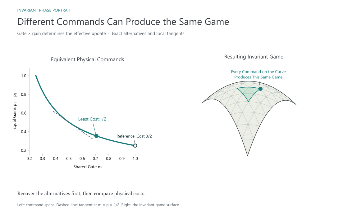
The command that changes a game need not be unique. Different settings may produce the same payoff tensor or agree only in selected invariant measurements. Recovering those alternatives lets us choose among interventions by cost or by constraints on the physical controls.

Problem. Given a successful command, recover commands with the same measured effect and find a lower-cost member where the available solver can certify one.

Procedure.

1. Evaluate the reference command.
2. Pull equality with the reference measurements back through the command-to-game map.
3. Intersect with the permitted command region. These equations define the finite alternatives.
4. Differentiate the same measurement map to obtain local directions that preserve the measurements to first order.

Code. reference_command is a command vector, and measurements specifies which distinctions to retain. Equality of selected invariants can be coarser than equality of games up to relabeling.

alternatives = problem.equivalent_to(reference_command, measurements)
values = problem.games.then_apply(measurements)
direction, nullspace, residual = local_controls(values, command, desired_change)

Example: A Shared Gate and Two Independent Gains

Keep the three-individual payoff family and target. Replace the direct actuator with a gate \(m\) and gains \(p_1,p_2\). The effective changes are

\[ v_1=mp_1 \qquad v_2=mp_2 \qquad 0\le m,p_1,p_2\le1 \]

The command \((1,1/4,1/4)\) reproduces the successful game from inverse design. Suppose physical cost is \(m+p_1+p_2\). We want cheaper commands with the same invariant vector.

Recover the Fiber and Minimize Cost Along the Curve

product_transfers = Map(lambda command: command[..., :1] * command[..., 1:])
product_parameters = product_transfers.then_apply(project_parameters)
product_allowed = (
    ge(Map(lambda v: v), 0) & ge(Map(lambda v: 1 - v), 0)
    & project_allowed.pullback(product_transfers)
)
product_control = Control(product_parameters, product_allowed,
                          Map(lambda v: v.sum(axis=-1)), ("gate", "second_gain", "third_gain"))
product_problem = design(project_family, product_control, project_target)
product_values = product_problem.games.then_apply(project_measurements)
reference_command = exact([1, sp.Rational(1, 4), sp.Rational(1, 4)])
invariant_fiber = product_problem.equivalent_to(reference_command, project_measurements)
product_symbols = sp.symbols("m p1 p2", real=True)
fiber_equations = [expression for expression, relation in invariant_fiber.atoms(product_symbols) if relation == "eq"]
fiber_solutions = sp.solve(fiber_equations, product_symbols[1:], dict=True)
fiber_curve = rational_map([product_symbols[0], *[fiber_solutions[0][s] for s in product_symbols[1:]]], (product_symbols[0],))
fiber_minimum = rational_curve_minimum(
    product_problem, fiber_curve, product_symbols[0], sp.Interval(0, 1)
)
fiber_command = product_problem.select(fiber_minimum["command"])
fiber_verified = fiber_minimum["verified"] and fiber_command.verify()
local_command = torch.tensor([.5, .5, .5], dtype=torch.float64)
local_direction, local_nullspace, local_residual = local_controls(
    product_values, local_command, torch.zeros(3, dtype=torch.float64)
)
local_jacobian = torch.func.jacfwd(product_values)(local_command)
finite_null_step = local_command + .1 * local_nullspace[:, 0]
finite_measurement_change = product_values(finite_null_step) - product_values(local_command)
zero_product_jacobian = torch.func.jacfwd(product_values)(torch.zeros(3, dtype=torch.float64))

Solution. Symbolic evaluation and equality with the reference measurements produce

\[ mp_1=mp_2=\frac14 \qquad (p_1,p_2)=\left(\frac1{4m},\frac1{4m}\right) \qquad \frac14\le m\le1 \]

The cost along this recovered curve is \(m+1/(2m)\). The one-variable procedure isolates the stationary points and compares their costs with both endpoints. The minimum is

\[ m=\frac1{\sqrt2} \qquad p_1=p_2=\frac1{2\sqrt2} \qquad c=\sqrt2 \]

This certifies minimum cost on the recovered equivalence curve. The original command costs \(3/2\). Both commands produce the same payoff tensor in this family, although the equality constraints were stated through invariant measurements.

Torch also differentiates the composed map. At a regular point, the Jacobian nullspace gives the tangent direction to this curved set. A finite step along that tangent generally leaves the set. At the all-zero command the Jacobian vanishes, even though simultaneous nonzero gate and gain can change the game. These are limits of first-order information, which the exact equations retain.

7. Equilibrium and Dynamics: Behavioral Consequences of Changing Payoffs

Figure 7: Consider the successful three-individual game returned by inverse design. The invariant description is fixed, while two initial action profiles lead to different outcomes under the same supplied update rule. The response paths show action states, rather than additional games in invariant space.

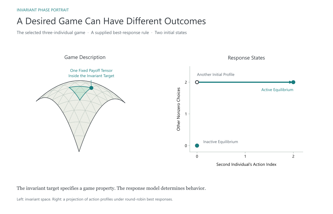
Changing a game changes the incentives available to individuals. Predicting what the individuals do also requires a response model and an initial state. An invariant target alone does not specify a selection rule among equilibria or a learning process.

Problem. After selecting a game in the invariant target, compute the consequences under supplied behavioral assumptions.

Procedure.

1. Evaluate the selected intervention to obtain the game.
2. Check equilibrium conditions directly on that payoff tensor.
3. For dynamics, supply the state, the response rule, and any update schedule, then apply the rule repeatedly.

The invariant map continues to describe the game being played. The trajectory describes the response state.

Code. intervention retains the selected command and game. initial is a behavioral state, schedule chooses an update, and response_step maps the current state and update to the next state under that game.

game = intervention.game()
equilibria = pure_equilibria(game)
trajectory = rollout(initial, schedule, partial(response_step, game), steps)

Example: Two Outcomes in the Same Desired Game

Use the game computed in inverse design, with joint weights \((1/2,1/4,1/4)\). Suppose individuals update in a fixed round-robin order. At each update, the selected individual chooses a best response to the others’ current choices and keeps the current action when that action ties for best.

Evaluate Equilibria and the Supplied Response Model

response_game = project_solution.game()
response_equilibria = pure_equilibria(response_game)
response_initials = ((0, 0, 0), (1, 0, 1))
response_traces = [
    rollout(profile, round_robin, partial(best_response_step, response_game), 6)
    for profile in response_initials
]
response_target_verified = project_target.contains(response_game)
response_coordinates = project_measurements(response_game)

Solution. Enumerating unilateral payoff comparisons gives two pure equilibria, written here as action indices

\[ (0,0,0) \qquad (1,2,1) \]

The second profile corresponds to effort values \((1,2,2)\). Starting from \((0,0,0)\), every update leaves the state unchanged. Starting from \((1,0,1)\), the second individual’s first update reaches \((1,2,1)\). Throughout both runs, the invariant vector remains \((1/12,1/24,1/24)\) because the payoff tensor remains fixed.

This gives the requested hook for a behavioral model. A different learning or evolutionary rule can replace the response step. Claims about the resulting path or terminal behavior must then follow from that supplied rule and state space.

8. Temporary Control: Reaching a State Where Intervention Can End

Figure 8: Consider a temporary intervention that helps a system leave an inactive response state. The added own-action term leaves the target’s three-way invariants unchanged. The lower path shows the controlled response reaching a state from which the original game reaches the active equilibrium without further intervention.

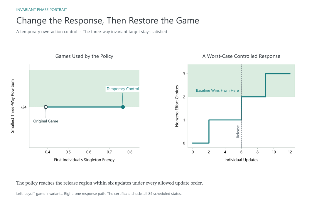
A controller may want to change behavior temporarily and then restore the original game. Knowing that a target state is reachable while control remains active does not establish that withdrawal will succeed. We need states from which the baseline dynamics already guarantees the desired outcome.

Problem. Find a policy that reaches a release region, then stops intervening while the baseline dynamics completes the transition.

Procedure.

1. Compute backward reachability under the baseline game. This identifies states from which every permitted update sequence reaches the behavioral goal.
2. Compute backward reachability to that region using the available interventions.
3. Retain commands that decrease the resulting layer rank.
4. Check separately that every game used by the policy satisfies the invariant target.

Code. states contains the complete finite response state, including any scheduling memory. successors(state, command) returns every allowed next state. baseline_actions permits only the zero command, while actions includes temporary controls.

baseline_layers, baseline_policy = winning_layers(
    states, baseline_actions, successors, safe, goal
)
release = baseline_layers[-1]
controlled_layers, controlled_policy = winning_layers(
    states, actions, successors, safe, release
)

Example: Activate the Running Game and Withdraw

Use the selected three-individual game again. Add an instrument \(s x_0\) to the first individual’s payoff, with \(s\) either \(0\) or \(1/2\). Such an own-action term leaves every three-way contrast unchanged. Both available games therefore satisfy the same invariant target.

Suppose each individual updates once per round, in any order. The controller observes the current profile and which individuals still need to update. Including that scheduling mask gives \(12\times7=84\) states. We seek eventual arrival at the active equilibrium \((1,2,1)\), starting from inactivity.

Construct the Successor Relation and Release Policy

activation_effect = exact(np.zeros((3,) + project_shape, dtype=int))
activation_effect[0] = efforts[0]
activation_change = polynomial([((1,), activation_effect)])
activation_games = response_game.with_payoff_rule(partial(add_payoff_terms, activation_change))
activation_levels = (sp.S.Zero, sp.Rational(1, 2))
activation_states = tuple(product(product(*(range(size) for size in project_shape)), range(1, 8)))
activation_successors = partial(scheduled_responses, activation_games)


def baseline_choices(state):
    return (sp.S.Zero,)


def activation_choices(state):
    return activation_levels


activation_safe = set(activation_states)
activation_goal = {state for state in activation_states if state[0] == (1, 2, 1)}
baseline_layers, baseline_policy = winning_layers(
    activation_states, baseline_choices, activation_successors, activation_safe, activation_goal
)
release_profiles = {
    profile for profile in product(*(range(size) for size in project_shape))
    if all((profile, phase) in baseline_layers[-1] for phase in range(1, 8))
}
release_states = {state for state in activation_states if state[0] in release_profiles}
activation_layers, activation_policy = winning_layers(
    activation_states, activation_choices, activation_successors, activation_safe, release_states
)
activation_start = ((0, 0, 0), 7)
activation_rank = next(i for i, layer in enumerate(activation_layers) if activation_start in layer)
activation_preserves_target = all(project_target.contains(activation_games(exact([s]))) for s in activation_levels)
activation_measurements = [project_measurements(activation_games(exact([s]))) for s in activation_levels]

Solution. The baseline calculation finds seven profiles that reach the active equilibrium under every scheduling phase. These are exactly the profiles with at least two individuals choosing nonzero effort. We use that phase-independent set as the release region.

The second calculation reaches this region from \((0,0,0)\) in at most six individual updates, under every allowed update order. The retained commands define the policy. After entry, set \(s=0\) and follow the baseline dynamics. The original payoff game is restored, and the response still reaches the active equilibrium.

The certificate concerns the stated finite response model, including the tie rule and fair-round scheduler. The invariant calculation supplies a separate guarantee: the selected three-way target holds for every game used along the policy.

9. Distributed Control: Invariant Targets in Larger Games

Figure 9: Consider two larger systems: six individuals connected by configurable pair terms, and four individuals choosing policies in a shared environment. The network panel shows two selected invariant coordinates and the effect of targeted versus uniform controls. The policy panel shows the limiting four-way alignment measurement along a control curve. Both targets are computed from the full payoff tensors.

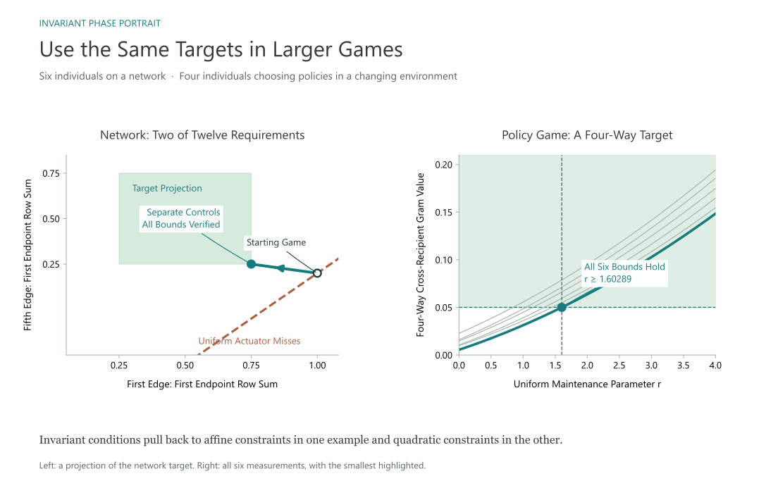
The preceding examples use small tensors so that the whole calculation can be inspected. The same construction applies when many individuals interact or when a simulation supplies the payoff table. The central question remains which permitted parameter choices place the resulting invariant vector in the target.

Problem. Allocate control across a larger system, or tune a model that generates a game, while retaining an invariant target and the resulting constraints.

Procedure.

1. Supply a payoff model with the required action counts.
2. Measure the interaction channels relevant to the target and pull their requirements back through the control map.
3. Inspect the resulting constraints before choosing a solver. Affine constraints admit the same certified solver as before. Nonlinear constraints need an applicable nonlinear procedure.

Code. family can be a direct tensor formula or a model compiled from policy profiles. The composition and target interface remain unchanged.

problem = design(family, control, desired_type.pullback(measurements))

Example: Six Individuals and Separate Network Controls

Consider six individuals with binary settings, arranged on a cycle. Each edge contributes a score \(x_i x_j\) to the two endpoint payoffs, weighted by \(a_e\) and \(1-a_e\). Add a fixed three-way term involving individuals \(0,2,4\), with different signs across recipients. The game therefore contains both pairwise and higher-order structure.

For each edge, require both endpoint recipients to have a Gram row sum of at least \(1/4\) in that edge’s interaction block. This asks for a minimum contribution to the combined pair response. The three-way term remains present and outside this particular target.

Build the Tensor and Solve the Network Control Problem

network_shape = (2,) * 6
network_actions = np.meshgrid(*[exact([-1, 1])] * 6, indexing="ij")
network_edges = ((0, 1), (1, 2), (2, 3), (3, 4), (4, 5), (0, 5))
network_weights = exact([1, sp.Rational(4, 5), sp.Rational(1, 2), sp.Rational(9, 10), sp.Rational(1, 5), sp.Rational(3, 5)])
network_base = -np.stack(network_actions) * sp.Rational(1, 4)
network_terms = []
for edge_index, (i, j) in enumerate(network_edges):
    feature = network_actions[i] * network_actions[j]
    network_base[j] += feature
    coefficient = exact(np.zeros((6,) + network_shape, dtype=int))
    coefficient[i], coefficient[j] = feature, -feature
    powers = tuple(int(k == edge_index) for k in range(6))
    network_terms.append((powers, coefficient))
network_base += exact([1, -1, 0, 1, 0, -1])[:, None, None, None, None, None, None] * (
    network_actions[0] * network_actions[2] * network_actions[4] / 3
)
network_change = polynomial(network_terms)
network_family = Game(network_base, network_shape).with_payoff_rule(partial(add_payoff_terms, network_change))
network_rows = tuple(tuple(gram(edge, p, q) for q in range(6)) for edge in network_edges for p in edge)
network_measurements = Map(lambda game: stack([sum(f(game) for f in row) for row in network_rows], axis=-1))
network_target = ge(network_measurements, sp.Rational(1, 4))
network_parameters = Map(lambda v: like(network_weights, v) - v[..., :6])
network_bounds = (
    ge(network_parameters, 0) & ge(Map(lambda v: 1 - network_parameters(v)), 0)
    & ge(Map(lambda v: v[..., 6:] - v[..., :6]), 0)
    & ge(Map(lambda v: v[..., 6:] + v[..., :6]), 0)
)
network_control = Control(network_parameters, network_bounds, Map(lambda v: v[..., 6:].sum(axis=-1)),
                          tuple([f"edge_{i}" for i in range(6)] + [f"cost_{i}" for i in range(6)]))
network_problem = design(network_family, network_control, network_target)
network_symbols = sp.symbols("v0:6 c0:6", real=True)
network_answer = solve_affine(network_problem, network_symbols)
network_selected = network_problem.select(exact(network_answer.data["point"]))
uniform_parameters = Map(lambda v: like(network_weights, v) - v[..., :1])
uniform_bounds = ge(uniform_parameters, 0) & ge(Map(lambda v: 1 - uniform_parameters(v)), 0)
uniform_control = Control(uniform_parameters, uniform_bounds, Map(lambda v: v.sum() * 0), ("uniform_change",))
uniform_answer = solve_affine(design(network_family, uniform_control, network_target), (sp.Symbol("v", real=True),))
network_verified = network_answer.verify() and network_selected.verify() and uniform_answer.verify()
network_sensitivity = torch.func.jacfwd(network_problem.games.then_apply(network_measurements))(
    torch.zeros(12, dtype=torch.float64)
)

Solution. There are \(64\) joint action profiles and \(384\) payoff entries. Applying the invariant map yields the edge conditions

\[ \frac14\le a_e\le\frac34 \]

The starting weights are \((1,4/5,1/2,9/10,1/5,3/5)\). With independently adjustable edges and total absolute adjustment as cost, the solver returns

\[ v^*=\left(\frac14,\frac1{20},0,\frac3{20},-\frac1{20},0\right) \qquad c(v^*)=\frac12 \]

Here \(a'_e=a_e-v_e\). The commands reduce excessive weights and increase a deficient weight. The result satisfies all twelve invariant requirements and has a checked minimum-cost certificate.

A uniform adjustment cannot succeed. The first edge requires \(v\ge1/4\), while the fifth requires \(v\le-1/20\). The solver certifies this contradiction after substituting the uniform actuator into the same invariant target. No action relabelings need to be enumerated.

Example: Four Individuals Choosing Policies

Now consider four individuals using a shared facility. Each chooses one of three policies: operate, maintain, or operate only when capacity is sufficiently high. Capacity changes with joint usage and random wear. The model specifies the state transitions and each individual’s reward over five periods.

Enumerating the \(3^4=81\) policy profiles and taking expected discounted rewards produces a payoff tensor with \(324\) entries. A uniform maintenance parameter \(r\) changes the rewards. We ask for every pair of recipients to have four-way alignment at least \(1/20\)

\[ M_{\{0,1,2,3\}}[p,q]\ge\frac1{20} \qquad p<q \qquad 0\le r\le4 \]

Supply the Environment and Derive the Feasible Parameter Region

policy_shape = (3, 3, 3, 3)
operating_values = exact([1, sp.Rational(6, 5), sp.Rational(4, 5), sp.Rational(11, 10)])
maintenance_costs = exact([sp.Rational(2, 5), sp.Rational(3, 5), sp.Rational(4, 5), 1])


def policy_actions(profile, capacity):
    return tuple(int(policy == 0 or (policy == 2 and capacity >= 3)) for policy in profile)


def facility_transition(theta, time, profile):
    matrix = exact(np.zeros((5, 5), dtype=int))
    for capacity in range(5):
        active = sum(policy_actions(profile, capacity))
        for wear, probability in ((0, sp.Rational(3, 4)), (1, sp.Rational(1, 4))):
            following = max(0, min(4, capacity + 4 - 2 * active - wear))
            matrix[capacity, following] += probability
    return like(matrix, theta)


def facility_reward(theta, time, profile):
    base = exact(np.zeros((4, 5, 5), dtype=int))
    maintenance = exact(np.zeros((4, 5, 5), dtype=int))
    for capacity in range(5):
        actions = policy_actions(profile, capacity)
        for individual, action in enumerate(actions):
            if action:
                base[individual, capacity, :] = operating_values[individual] * sp.Rational(capacity, max(1, sum(actions)))
            else:
                base[individual, capacity, :] = -maintenance_costs[individual]
                maintenance[individual, capacity, :] = 1
    return like(base, theta) + theta[..., :, None, None] * like(maintenance, theta)


compiled_family = policy_game(policy_shape, exact([0, 0, 0, 0, 1]), facility_transition,
                              facility_reward, 5, sp.Rational(9, 10))
# Fixed transitions and affine rewards make this exact coefficient cache valid.
policy_base = compiled_family(exact([0, 0, 0, 0]))
policy_coefficients = [compiled_family(exact([int(i == j) for i in range(4)])).payoffs - policy_base.payoffs for j in range(4)]
policy_change = polynomial([(tuple(int(i == j) for i in range(4)), coefficient)
                            for j, coefficient in enumerate(policy_coefficients)])
policy_family = policy_base.with_payoff_rule(partial(add_payoff_terms, policy_change))
policy_parameters = Map(lambda r: r[..., :1] * like([1, 1, 1, 1], r))
policy_measurements_list = tuple(gram((0, 1, 2, 3), i, j) for i, j in combinations(range(4), 2))
policy_measurements = Map(lambda game: stack([f(game) for f in policy_measurements_list], axis=-1))
policy_target = ge(policy_measurements, sp.Rational(1, 20))
policy_control = Control(policy_parameters,
                         ge(Map(lambda r: r), 0) & ge(Map(lambda r: 4 - r), 0),
                         Map(lambda r: 4 * r[..., 0]), ("maintenance_rate",))
policy_problem = design(policy_family, policy_control, policy_target)
rate_symbol = sp.Symbol("r", real=True)
policy_rate_region = univariate_region(policy_problem.feasible, rate_symbol, sp.Interval(0, 4))
policy_command = exact([policy_rate_region.start])
policy_selected = policy_problem.select(policy_command)
policy_verified = policy_selected.verify()
policy_polynomials = [sp.factor(z) for z in policy_measurements(policy_problem.games(exact([rate_symbol])))]
policy_interior = exact([(policy_rate_region.start + policy_rate_region.end) / 2])
policy_interior_game = policy_problem.games(policy_interior)
policy_adaptive_equilibrium = ge(deviation_gaps((2, 2, 2, 2)), sp.Rational(1, 20)).contains(policy_interior_game)
policy_sensitivity = torch.func.jacfwd(policy_problem.games.then_apply(policy_measurements))(
    torch.tensor([float(policy_interior[0])], dtype=torch.float64)
)

The environment transitions are independent of the reward parameter, and the rewards depend affinely on that parameter. Evaluating the zero vector and the four unit vectors therefore constructs an exact affine coefficient cache for the payoff model. Torch differentiates this same tensor formula. The Gram measurements remain quadratic functions of the parameter.

Solution. The one-variable solver intersects the six quadratic inequalities with the allowed parameter interval. The output is a closed interval \([r_{\min},4]\), with \(r_{\min}\approx1.60289\) and an exact algebraic lower endpoint. Minimizing cost \(4r\) selects that endpoint. The returned game is checked against every original invariant comparison.

A separate check of the all-adaptive policy profile fails the specified strict-equilibrium margin at an interior successful parameter. Thus the model reaches the requested four-way invariant type without establishing that every individual will choose the adaptive policy. Such a behavioral requirement can be added explicitly, using the same payoff tensor.

10. Information Sufficiency

Figure 10: Consider two possible games that differ only in the sign of a three-way effect. All quadratic invariant measurements agree, but the two games need different commands to reach the specified invariant target. A cubic measurement separates the two points and supports a successful decision.

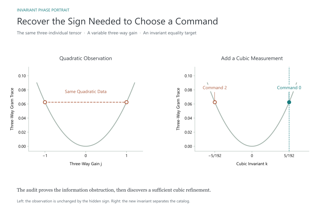
The previous examples assume enough information to evaluate the current game. Suppose instead that a controller receives only selected invariant measurements. Two possible games may produce the same observation while requiring different interventions. We can test whether the available information supports a guaranteed decision.

Problem. Determine whether each observation class admits a command that succeeds for every game in that class. If not, search a supplied collection of additional measurements for a useful refinement.

Procedure.

1. Use the same control construction to obtain each possible game’s successful-command region.
2. Group games with equal observations and intersect the regions within each group.
3. Check the intersections. A checked empty intersection is an information obstruction when the individual games are reachable.
4. Refine the observations and repeat until every remaining class has a checked successful command or the supplied search is exhausted.

Code. games is a finite catalog of possible current games. problems contains their control problems in common command coordinates. measurements contains the available observation functions, and candidates generates additional invariant measurements.

audit = audit_observations(games, problems, measurements, symbols)
measurements, audit, status = refine_observations(
    games, problems, measurements, candidates, symbols
)

Example: A Hidden Sign in the Three-Individual Game

Take the successful game from inverse design as a reference. Introduce a parameter \(j\) that multiplies only the three-way contrast, leaving every lower-order effect fixed. The current value is either \(+1\) or \(-1\). A command \(v\in[0,2]\) changes the gain to \(j+v\).

This question uses a finer invariant target than the earlier row-sum thresholds. Require a cubic contraction to equal the reference value. One such contraction averages the product of the first individual’s singleton effect, the complementary pair effect, and the three-way effect

\[ k(u)=\left\langle T_{\{0\},0}T_{\{1,2\},0}T_{\{0,1,2\},0}\right\rangle \qquad k(u)=k(u_{\mathrm{reference}}) \]

On this family the first two factors remain fixed, so this invariant is linear in the three-way gain. The desired region is defined by an invariant equality, while the observation set can initially be much coarser.

Audit the Observations and Discover a Refinement

information_reference = project_solution.game()
information_joint = effect(information_reference, (0, 1, 2))
information_change = polynomial([((0,), -information_joint), ((1,), information_joint)])
information_family = information_reference.with_payoff_rule(partial(add_payoff_terms, information_change))
information_games = [information_family(exact([j])) for j in (1, -1)]
reference_witness = moment(((0,), 0), ((1, 2), 0), ((0, 1, 2), 0))
information_target = eq(reference_witness, reference_witness(information_reference))


def coupling_update(start, command):
    return like([start], command) + command


information_allowed = ge(Map(lambda v: v), 0) & ge(Map(lambda v: 2 - v), 0)
information_controls = [Control(Map(partial(coupling_update, j)), information_allowed,
                               Map(lambda v: v.sum(axis=-1)), ("joint_gain_change",)) for j in (1, -1)]
information_problems = [design(information_family, control, information_target) for control in information_controls]
information_symbols = (sp.Symbol("v", real=True),)
quadratic_observations = [gram(S, p, q) for S in subsets(3) for p in range(3) for q in range(p, 3)]
information_audit = audit_observations(information_games, information_problems, quadratic_observations, information_symbols)
refined_observations, refined_audit, information_status = refine_observations(
    information_games, information_problems, quadratic_observations,
    islice(moment_candidates(3, 3), 3000), information_symbols
)
information_commands = [answer.data["point"] for indices, answer in refined_audit]
information_separator_values = [refined_observations[-1](game) for game in information_games]

Solution. Every quadratic Gram entry agrees between the two possible games. Their successful-command regions are respectively \(\{0\}\) and \(\{2\}\), so no command succeeds for the whole observation class. The procedure verifies both individual reachability and the empty common intersection.

Searching invariant products through degree three discovers a separator with values \(+5/192\) and \(-5/192\). The refined observations split the catalog into two classes. The procedure then returns command \(0\) for the positive class and command \(2\) for the negative class.

This certifies sufficiency for the supplied catalog and control problems. A finite catalog cannot establish a sufficient statistic for all games of the same shape. The general lesson is the algorithmic test: measurements are adequate for a decision when every observation class has a common successful intervention.

Conclusion

The preceding posts supplied invariant descriptions of games. Here, the same invariant descriptions can be used to intervene on games to change the game type. Next steps in this vein will likely include more in-depth game decompositions and also analysis of the space of games.

Appendix: Atomic Operations

Here, we build the specific operations needed to describe and control games. The forward direction takes parameters to payoffs, separates the payoffs into interaction effects, and computes invariant measurements. The backward direction starts with desired properties and turns them into conditions on parameters and interventions.

Each operation below has a mathematical definition and a matching implementation. Some are basic operations, while others are procedures built by composing those operations. They share the objects defined first, so we can combine them to search for interventions, certify what the controls can achieve, check intervention paths, and construct policies under a supplied dynamics model.

Shared Objects and Setup

I⁴ will use a similar approach to software architecture as in the game and agent library, the differential-game implementation, and the CIT library. The guiding principles are to keep the data small, represent operations as functions, and compose them.

The code blocks below share these imports:

from dataclasses import dataclass
from functools import partial, reduce
from itertools import (
    combinations,
    combinations_with_replacement,
    islice,
    permutations,
    product,
)
from math import prod
from operator import and_, mul
from typing import Callable
import numpy as np
import sympy as sp
import torch
from scipy.optimize import linprog

A Map evaluates a supplied function with evaluate(values) and composes that function with another map using then_apply(next_map). If f maps parameters to games and g measures games, f.then_apply(g) measures the game produced by those parameters.

def compose_maps(first, second, values):
    return second(first(values))


@dataclass(frozen=True)
class Map:
    function: Callable

    def evaluate(self, values):
        return self.function(values)

    def __call__(self, values):
        return self.evaluate(values)

    def then_apply(self, next_map):
        return Map(partial(compose_maps, self, next_map))

Game holds the payoffs and action counts. In code, payoffs has shape (..., n, m1, ..., mn), with optional leading batch dimensions. The with_payoff_rule method binds a supplied payoff rule to that game. The rule receives the base payoffs and the parameters and returns the new payoff tensor. Thus, we can alter selected entries, add interaction effects, or replace the payoffs through an outcome model.

@dataclass(frozen=True)
class Game:
    payoffs: torch.Tensor | np.ndarray
    shape: tuple

    def with_payoff_rule(self, payoff_rule):
        return Map(partial(instantiate_game, self, payoff_rule))

    def relabel(self, permutations):
        u = self.payoffs
        for i, order in enumerate(permutations):
            index = [slice(None)] * u.ndim
            index[u.ndim - len(self.shape) + i] = list(order)
            u = u[tuple(index)]
        return Game(u, self.shape)


def instantiate_game(base, payoff_rule, theta):
    return Game(payoff_rule(like(base.payoffs, theta), theta), base.shape)

We instantiate a particular game by evaluating the family at chosen parameter values, and evaluating a candidate intervention gives the resulting game.

base = Game(payoffs, action_sizes)
family = base.with_payoff_rule(payoff_rule)
parameters = Map(lambda command: psi(theta0, command))
controlled_games = parameters.then_apply(family)

starting_game = family.evaluate(theta0)
resulting_game = controlled_games.evaluate(command)

The target checks below determine whether the intervention is successful.

For example, payoff_rule(u, theta) might evaluate a physical outcome model and then each individual’s utility. Another parameterization can use the same base. Another control map can use the same family. Composing several parameter maps works the same way:

controlled_games = instruments.then_apply(parameters).then_apply(family)

We can also evaluate the same formulas symbolically. Torch tensors carry numerical values and derivatives, and NumPy object arrays carry the corresponding exact SymPy entries. The small array adapters below preserve these two kinds of arithmetic. Exact inputs use integers or rationals, and an arbitrary Torch-only simulator supplies a differentiable family, but symbolic claims require a model that also supports the exact operations used below.

def exact(values):
    array = np.asarray(values, dtype=object)
    return np.array([sp.sympify(v) for v in array.flat], dtype=object).reshape(
        array.shape
    )


def like(values, x):
    if isinstance(x, torch.Tensor):
        if isinstance(values, torch.Tensor):
            return values.to(x)
        return x.new_tensor(np.asarray(values, dtype=float))
    return exact(values)


def stack(values, axis=0):
    if isinstance(values[0], torch.Tensor):
        return torch.stack(values, dim=axis)
    return np.stack(values, axis=axis)


def average(x, axes, keepdims=False):
    size = prod(x.shape[i] for i in axes)
    total = x.sum(axis=axes, keepdims=keepdims)
    return total / size if isinstance(x, torch.Tensor) else total * sp.Rational(1, size)

The symbolic branch of average keeps division exact by using sp.Rational. This matters for the certificate checks below, which verify algebraic equalities without rounding error.

1. Instantiate a Game

Goal: Obtain the game associated with a chosen set of model parameters.

Inputs: A parameter vector \(\theta \in \Theta \subseteq \mathbb{R}^d\), collecting values for the \(d\) model parameters, and a payoff function \(\varphi\) from \(\Theta\) to \(V\). Here \(\Theta\) is the set of allowed parameter settings, and \(\varphi\) specifies the payoffs at each setting.

Outputs: A payoff tensor \(u = \varphi(\theta) \in \mathbb{R}^{n \times m_1 \times \cdots \times m_n}\), where \(n\) is the number of individuals and \(m_i\) is the number of actions available to individual \(i\). The tensor stores one payoff table per individual. To retrieve a payoff, specify the recipient and the action chosen by each individual.

A payoff model for a game maps parameter values to payoffs.

\[ \Theta \xrightarrow{\varphi} V \]

Such a model may be assembled from an outcome map and a utility map, or given directly as a payoff formula. For a polynomial model, collect the coefficients into payoff tensors:

\[ \varphi(\theta) = \sum_\alpha U_\alpha \theta^\alpha \]

Here \(\theta^\alpha = \prod_j \theta_j^{\alpha_j}\). Linear terms describe separate parameter effects. Products involving different parameters describe how those effects interact. The polynomial evaluator handles both forms.

def evaluate_polynomial(terms, theta):
    result = 0
    for powers, coefficient in terms:
        monomial = reduce(mul, (theta[..., j] ** k for j, k in enumerate(powers)), 1)
        if not isinstance(monomial, torch.Tensor):
            monomial = np.asarray(monomial, dtype=object)
        array = like(coefficient, theta)
        result = result + monomial[(...,) + (None,) * array.ndim] * array
    return result


def polynomial(terms):
    terms = tuple(terms)
    return Map(partial(evaluate_polynomial, terms))

Thus a supplied collection of coefficient tensors can be attached to the base game:

change = polynomial(terms)
family = base.with_payoff_rule(lambda u, theta: u + change(theta))
controlled_games = parameters.then_apply(family)

Alternatively, base.with_payoff_rule(lambda u, theta: change(theta)) specifies the entire payoff rule. Tensor evaluation preserves the Torch graph, and evaluation at a vector of symbols produces exact payoff expressions from the same rule.

We can also choose the group that determines what counts as the same description. Here the relabeling group is

\[ G = \prod_i S_{m_i} \]

Each permutation changes an individual’s action labels. The group acts on the tensor by reordering action axes, as in Game.relabel. Individuals and payoff units remain fixed. This determines the invariant ring

\[ \mathbb{R}[V]^G = \{f \in \mathbb{R}[V] : f(\sigma \cdot u) = f(u) \text{ for all } \sigma \in G\} \]

The code’s permutation arrays list old indices in their new order. A named action in a target must be transported with this reordering. Likewise, a relabeled control problem must transport the relevant payoff rule and permissions to the invariant ring representation.

2. Decompose Payoffs into Interaction Effects

Goal: Separate individual and joint contributions to payoffs so we can examine which interactions shape the game.

Inputs: A payoff tensor \(u \in V\), containing the individuals’ payoffs for every joint action, and a subset \(S\) of individuals whose interaction we want to examine.

Outputs: The projection \(P_Su\), an interaction tensor isolating the joint effect of the actions belonging to \(S\). The tensor retains a payoff for each recipient, averages over actions outside \(S\), and removes effects attributable to smaller subsets. Summing these tensors over all subsets reconstructs \(u\).

We use the contrast-block decomposition from the invariant coordinates post, which separates mean payoffs, individual effects, and interactions among subsets of individuals. Algebraically, this is a factorial ANOVA decomposition.⁵

To isolate dependence on individual \(i\)’s action, first average the payoffs over all actions available to \(i\), holding the other individuals’ actions fixed. Subtracting the average gives the payoff variation associated with \(i\)’s action:

\[ (\mathsf{A}_i f)(a) = \frac{1}{m_i} \sum_{b_i \in A_i} f(b_i, a_{-i}) \]

The remaining contrast is \(\mathsf{C}_i f = f - \mathsf{A}_i f\). Averaging twice changes nothing (averaging is idempotent). Thus \(\mathsf{A}_i\) and \(\mathsf{C}_i\) are complementary projections, and operators on different axes commute. For an interaction subset \(S\), take contrasts on the axes in that subset and averages on the others:

\[ P_S = \prod_{i \in S} \mathsf{C}_i \prod_{i \notin S} \mathsf{A}_i \]

Write \(T_{S, p} = P_S u_p\). The empty subset gives the mean, singleton subsets give individual effects, and larger subsets give irreducible joint effects. Expanding \(\prod_i(\mathsf{A}_i + \mathsf{C}_i)\) proves reconstruction:

\[ u_p = \sum_{S \subseteq [n]} T_{S, p} \]

The implementation is successive averaging and subtraction. Averaged-out axes retain length one, so broadcasting reconstructs the full table without repeating constant entries.

def subsets(n):
    return (S for k in range(n + 1) for S in combinations(range(n), k))


def effect(game, S):
    u = game.payoffs
    for i in range(len(game.shape)):
        axis = u.ndim - len(game.shape) + i
        mean = average(u, (axis,), keepdims=True)
        u = u - mean if i in S else mean
    return u


def recipient(u, p, n):
    return u[(..., p) + (slice(None),) * n]

For example, the same projected tensor can be read by interaction or by recipient:

by_interaction = {S: effect(game, S) for S in subsets(len(game.shape))}
by_individual = {
    p: {S: recipient(block, p, len(game.shape))
        for S, block in by_interaction.items()}
    for p in range(len(game.shape))
}
reconstructed = sum(by_interaction.values())

These are two views of the same information. An interaction can affect individuals outside the interaction subset, so we keep the full recipient axis.

Figure 11: An individual’s payoff can depend on their own action, another individual’s action, or a combination of actions. Organizing those effects by payoff recipient gives the individual view. Organizing the same effects by the individuals whose actions are involved gives the interaction view. The diagram shows these two readings of one block array. Only selected interaction subsets are displayed, and each entry retains a full action-dependent tensor.

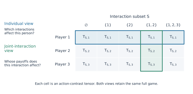
Use the uniform inner product \(\langle f, g \rangle = N^{-1} \sum_a f(a)g(a)\). The averaging projections are self-adjoint. If \(S \ne R\), an axis in their symmetric difference contributes \(\mathsf{A}_i\mathsf{C}_i = 0\), so

\[ \langle P_S f, P_R g \rangle = 0 \]

Consequently, \(\|u_p\|^2 = \sum_S \|T_{S, p}\|^2\). Changes in one interaction block don’t cancel a discrepancy in another (this will supply a control obstruction later).

The projections are equivariant, so relabeling and then projecting gives the same answer as projecting and then relabeling. Their entries are not themselves invariant.

The illustrative code computes requested blocks directly. A full compact contrast transform, as in the earlier post, stores all blocks in \(nN\) coefficients and avoids constructing \(2^n\) separate arrays.

3. Compute Game Invariants

Goal: Describe and compare games independently of the names attached to actions.

Inputs: A payoff tensor \(u \in V\) and either a polynomial \(f\) to average over the relabeling group \(G\) or a selection of interaction components to combine. The group \(G\) specifies which changes of action labels count as equivalent descriptions.

Outputs: An invariant measurement \(I_j \in \mathbb{R}[V]^G\), meaning a polynomial whose value is unchanged by the chosen relabelings, and the number \(I_j(u)\) obtained by evaluating that measurement on the game. Collecting \(r\) such values gives an invariant description \(I(u) \in \mathbb{R}^r\).

The projection onto the invariant ring acts on polynomial functions of games. This projection is the Reynolds average:

\[ (\mathcal{R}f)(u) = \frac{1}{|G|} \sum_{\sigma \in G} f(\sigma \cdot u) \]

Relabeling \(u\) permutes the summands, and averaging an invariant changes nothing. Therefore \(\mathcal{R}^2 = \mathcal{R}\). If we have an explicit list of relabelings, the implementation of this average is short:

def average_relabelings(function, relabelings, game):
    return sum(function(game.relabel(s)) for s in relabelings) / len(relabelings)


def reynolds(function, relabelings):
    return Map(partial(average_relabelings, function, relabelings))

The CIT library represents a polynomial by exponent tuples and exact coefficients. The same polynomial evaluator from operation 1 can read those terms against the flattened payoff tensor:

def flatten_payoffs(game):
    return game.payoffs.reshape((*game.payoffs.shape[: -len(game.shape) - 1], -1))


def payoff_polynomial(terms):
    return Map(flatten_payoffs).then_apply(polynomial(terms))

cit_measurement = payoff_polynomial(cit_polynomial.items())

If the supplied polynomial is invariant for this action, the polynomial can go directly into a target. Otherwise reynolds(cit_measurement, relabelings) constructs the invariant average of that polynomial. This explicit group enumeration is useful for small problems. We don’t need group enumeration for the contractions we use most often.

Since \(P_S\) commutes with relabeling and the uniform inner product is preserved, the Gram entry

\[ M_S[p, q] = \langle T_{S, p}, T_{S, q} \rangle \]

is invariant. The diagonal measures the size of an effect, and an off-diagonal entry measures agreement or opposition between two recipients within that interaction. Higher products give further invariant measurements:

\[ I_{(S_1, p_1), \ldots, (S_d, p_d)}(u) = \frac{1}{N} \sum_{a \in A} \prod_{j = 1}^d T_{S_j, p_j}(a) \]

A common relabeling permutes the profiles in this sum. Equivalently, this is the Reynolds average of the product evaluated at any fixed profile, because the group visits all profiles equally often.

def contract_moment(factors, game):
    n = len(game.shape)
    blocks = {S: effect(game, S) for S, p in factors}
    value = reduce(mul, (recipient(blocks[S], p, n) for S, p in factors))
    return average(value, tuple(range(value.ndim - n, value.ndim)))


def moment(*factors):
    factors = tuple((tuple(S), p) for S, p in factors)
    return Map(partial(contract_moment, factors))


def gram(S, p, q):
    return moment((S, p), (S, q))

For example, with a supplied subset, recipient pair, and contraction factors:

alignment = gram(S, p, q)
higher_order = moment(*factors)
controlled_alignment = controlled_games.then_apply(alignment)

Sums and products of these scalar functions remain invariants. They are ordinary maps, so a new invariant does not require a new target class or a new solver branch.

If we supply independent mixed strategies \(x_i\), weighted contraction gives the expected payoffs:

\[ \overline{u}_p(x) = \sum_{a \in A} u_p(a) \prod_i x_i(a_i) \]

def expected(game, strategies):
    values = game.payoffs
    for i in reversed(range(len(game.shape))):
        probability = like(strategies[i], values)
        weights = probability[(...,) + (None,) * (i + 1) + (slice(None),)]
        values = (values * weights).sum(axis=-1)
    return values

The strategy probabilities are nonnegative and sum to one on each action axis, and they must be relabeled alongside the game. The expectation describes the behavior, where uniform averaging in the invariant contractions defines structural measurements and does not presume uniform play.

4. Construct a Target Region

Goal: Express desired game properties as conditions we can test and solve.

Inputs: A reference game \(r \in V\) and a choice of structure to preserve, such as payoff ordering or unilateral incentives. Alternatively, supply measurement functions \(f_j\) from payoff tensors to real numbers, together with required values or lower bounds \(b_j\). These measurements can include the invariant contractions from operation 3. A positive margin \(\rho\) specifies how far required payoff advantages must stay from ties.

Outputs: A target region \(\mathcal{T} \subseteq V\), containing the games satisfying the requirements. Combining regions with & requires both properties. Combining regions with | allows either property. The reference-game constructor below generates the comparisons and alternative action labelings automatically.

A target is a region defined by equations and inequalities. Write the target requirements as

\[ h_j(u) = 0 \]

and

\[ g_k(u) \ge 0 \]

When these functions are invariant, the target is well-defined on relabeling classes. We can also use explicitly labeled payoff comparisons, provided their action witnesses move with a relabeling.

A Constraint stores one function and a relation to zero. A Region stores alternative clauses, each containing simultaneous constraints. A game belongs to the region when any clause holds. Intersection distributes over alternatives, and pullback substitutes the same map into every clause. The atoms method exposes the equations and inequalities of one clause for algebraic reasoning.

@dataclass(frozen=True)
class Constraint:
    value: Callable
    relation: str


@dataclass(frozen=True)
class Region:
    clauses: tuple = ((),)

    @property
    def branches(self):
        return tuple(Region((clause,)) for clause in self.clauses)

    @property
    def constraints(self):
        if len(self.clauses) != 1:
            raise ValueError(
                "Select a branch before extracting simultaneous constraints"
            )
        return self.clauses[0]

    def __and__(self, other):
        return Region(tuple(a + b for a in self.clauses for b in other.clauses))

    def __or__(self, other):
        return Region(self.clauses + other.clauses)

    def pullback(self, mapping):
        return Region(
            tuple(
                tuple(
                    Constraint(Map(mapping).then_apply(c.value), c.relation)
                    for c in clause
                )
                for clause in self.clauses
            )
        )

    def atoms(self, symbols):
        x = exact(symbols)
        return [
            (sp.expand(value), c.relation)
            for c in self.constraints
            for value in np.asarray(c.value(x), dtype=object).flat
        ]

    def contains(self, x):
        for clause in self.clauses:
            satisfied = True
            for constraint in clause:
                value = constraint.value(x)
                if not isinstance(value, torch.Tensor):
                    value = np.asarray(value, dtype=object)
                if constraint.relation == "eq" and not isinstance(value, torch.Tensor):
                    condition = np.asarray([
                        sp.sympify(entry).equals(0) is True for entry in value.flat
                    ])
                else:
                    condition = value == 0 if constraint.relation == "eq" else value >= 0
                satisfied = satisfied and bool(condition.all())
            if satisfied:
                return True
        return False


def subtract_target(target, measured):
    return measured - like(target, measured)


def ge(measure, lower):
    difference = Map(measure).then_apply(partial(subtract_target, lower))
    return Region(((Constraint(difference, "ge"),),))


def eq(measure, value):
    difference = Map(measure).then_apply(partial(subtract_target, value))
    return Region(((Constraint(difference, "eq"),),))

eq(measure, value) requires a measurement to equal the supplied value. ge(measure, lower) requires a measurement to meet a lower bound. Combining regions with & requires every condition to hold:

target = ge(alignment, tau) & ge(higher_order, eta)
cit_target = ge(cit_measurement, threshold)
parameter_region = target.pullback(family)
command_region = target.pullback(controlled_games)

To request a game type, supply one representative and choose which structure should agree:

reference = Game(reference_payoffs, action_sizes)
target = same_type_as(reference, preserve="preferences", margin=rho)
target = target & ge(alignment, tau)

Here reference_payoffs supplies a concrete payoff ordering. Ordinal ranks can serve as the entries when only ordering matters. The target constructor reads that ordering and generates conditions on the unknown game’s payoffs. The resulting payoffs may have entirely different values. The alignment requirement remains the invariant measurement defined earlier.

preserve	Structure retained from the reference game
"preferences"	Each individual’s ordering of all joint outcomes, including ties
"incentives"	Each individual’s ordering of actions for every fixed joint choice of the others
"payoffs"	Every payoff value, allowing action relabeling

All three choices identify independent action relabelings and keep individual identities fixed. The incentive choice preserves all unilateral payoff-comparison signs, including pure best responses and pure equilibria. Neither ordinal choice promises the same mixed equilibria. The payoff choice gives the exact relabeling orbit and needs no margin. A positive margin in the ordinal choices requires each strict advantage to be at least \(\rho\). Reference ties remain equalities.

For example, a representative Stag Hunt supplies a particular ordinal Stag Hunt subclass. A broader coordination target can instead specify equilibria and common preferences using the measurements below. Such a distinction separates the desired property from the names assigned to familiar examples.

For a fixed action labeling, let \(\mathcal{C}_{\rho}(r)\) contain the games satisfying the selected comparisons. Forgetting action names gives

\[ \mathcal{T}_{\rho}(r) = \bigcup_{\sigma \in G} \mathcal{C}_{\rho}(\sigma \cdot r) \]

Relabeling a candidate permutes these alternatives, so membership is invariant. For a separating invariant map \(I\), this also gives

\[ \mathcal{T}_{\rho}(r) = I^{-1}\bigl(I(\mathcal{T}_{\rho}(r))\bigr) \]

Thus the target defines a region in the same invariant quotient used above. We evaluate that region through payoff comparisons and group symmetry, without first expanding the region into polynomials in a complete set of invariant generators. Invariant thresholds and these compiled type requirements then compose through the same Region operations.

The implementation sorts reference payoffs within each comparison group. Equality between adjacent tied entries and a lower bound between adjacent distinct entries recover the full ordering by transitivity. Sorting happens once during target construction. Candidate payoffs remain differentiable tensor expressions.

def action_relabelings(shape):
    return product(*(permutations(range(size)) for size in shape))


def comparison_groups(shape, preserve):
    indices = np.arange(len(shape) * prod(shape)).reshape((len(shape), *shape))
    if preserve == "preferences":
        return tuple(tuple(row.flat) for row in indices)
    groups = []
    for p, size in enumerate(shape):
        for profile in product(*(range(m) for m in shape)):
            if profile[p] == 0:
                group = tuple(
                    indices[(p, *profile[:p], action, *profile[p + 1 :])]
                    for action in range(size)
                )
                groups.append(group)
    return tuple(groups)


def reference_comparisons(values, groups):
    ties, advantages = [], []
    for group in groups:
        ordered = sorted(group, key=values.__getitem__)
        for lower, higher in zip(ordered, ordered[1:]):
            if values[higher] == values[lower]:
                ties.append(tuple(sorted((higher, lower))))
            else:
                advantages.append((higher, lower))
    return tuple(sorted(ties)), tuple(sorted(advantages))


def payoffs_for_shape(shape, game):
    if game.shape != shape:
        raise ValueError("Reference and candidate must have the same action counts")
    return flatten_payoffs(game)


def compare_entries(shape, pairs, game):
    values = payoffs_for_shape(shape, game)
    return values[..., [a for a, b in pairs]] - values[..., [b for a, b in pairs]]


def same_type_as(reference, *, preserve="preferences", margin=None):
    if preserve not in ("preferences", "incentives", "payoffs"):
        raise ValueError("Choose preferences, incentives, or payoffs")
    if preserve != "payoffs" and (margin is None or margin <= 0):
        raise ValueError("Supply a positive margin for strict payoff advantages")
    if tuple(reference.payoffs.shape) != (len(reference.shape), *reference.shape):
        raise ValueError("Supply one reference game")
    groups = (
        comparison_groups(reference.shape, preserve) if preserve != "payoffs" else ()
    )
    target, seen = Region(()), set()
    for relabeling in action_relabelings(reference.shape):
        values = flatten_payoffs(reference.relabel(relabeling))
        if isinstance(values, torch.Tensor):
            values = values.detach().cpu().numpy()
        key = (
            tuple(values)
            if preserve == "payoffs"
            else reference_comparisons(values, groups)
        )
        if key in seen:
            continue
        seen.add(key)
        if preserve == "payoffs":
            branch = eq(Map(partial(payoffs_for_shape, reference.shape)), values)
        else:
            ties, advantages = key
            branch = eq(Map(partial(compare_entries, reference.shape, ties)), 0)
            branch = branch & ge(
                Map(partial(compare_entries, reference.shape, advantages)), margin
            )
        target = target | branch
    return target

The same constructor supports any finite shape \((m_1 \ldots m_n)\), including unequal action counts. The exhaustive implementation examines \(\prod_i m_i!\) relabelings and removes duplicate comparison patterns. Each ordinal branch uses at most \(n(N-1)\) comparisons. This supplies a general exact construction for modest games. Exhaustive relabeling becomes expensive as action counts grow. Direct invariant-property targets such as alignment bounds need no such enumeration. No catalog of named game types or user-supplied separating list is required.

Region() denotes no restrictions, and Region(()) denotes an empty target. contains checks one game or command. Numerical measurement maps retain their optional batch dimensions. The control solver below handles the alternative branches automatically.

Compute Incentive Gaps

Goal: Determine whether an individual would benefit from changing behavior while the others’ behavior stays fixed.

Inputs: A payoff tensor \(u \in V\) and designated behavior, including an action \(a_i\) for each individual, or a probability vector \(x_i \in \mathbb{R}^{m_i}\) describing how often each action is chosen. The entries of \(x_i\) are nonnegative and sum to one.

Outputs: A vector \(g(u) \in \mathbb{R}^{\ell}\) of incentive gaps, with one entry for each of the \(\ell\) payoff comparisons. Each entry subtracts the payoff from a unilateral alternative from the payoff under the designated behavior. Requiring \(g(u) \ge 0\) imposes the relevant equilibrium or dominance conditions.

For a designated profile \(a^*\) to be a pure equilibrium with margin \(\rho\), every unilateral deviation must satisfy

\[ u_i(a^*) - u_i(b_i, a^*_{-i}) \ge \rho \]

To make a designated action dominant, compare the designated action against every alternative at every opponents’ profile. Both are vectors of payoff differences:

def compute_deviation_gaps(profile, game):
    values = []
    for p, size in enumerate(game.shape):
        chosen = game.payoffs[(..., p, *profile)]
        for b in range(size):
            if b != profile[p]:
                alternative = (*profile[:p], b, *profile[p + 1 :])
                values.append(chosen - game.payoffs[(..., p, *alternative)])
    return (
        stack(values, axis=-1)
        if values
        else game.payoffs.reshape((*game.payoffs.shape[: -len(game.shape) - 1], -1))[
            ..., :0
        ]
    )


def deviation_gaps(profile):
    return Map(partial(compute_deviation_gaps, profile))


def compute_dominance_gaps(actions, game):
    gaps = []
    for profile in product(*(range(m) for m in game.shape)):
        for p, chosen in enumerate(actions):
            if profile[p] != chosen:
                preferred = (*profile[:p], chosen, *profile[p + 1 :])
                gaps.append(
                    game.payoffs[(..., p, *preferred)]
                    - game.payoffs[(..., p, *profile)]
                )
    return (
        stack(gaps, axis=-1)
        if gaps
        else game.payoffs.reshape((*game.payoffs.shape[: -len(game.shape) - 1], -1))[
            ..., :0
        ]
    )


def dominance_gaps(actions):
    return Map(partial(compute_dominance_gaps, actions))

equilibrium = ge(deviation_gaps(profile), rho)
dominance = ge(dominance_gaps(actions), rho)
target = equilibrium & ge(alignment, tau)

The symbolic path retains every inequality. The numerical path retains their derivatives. We do not reduce a vector of comparisons to a nonsmooth minimum before differentiation.

A supplied mixed profile is a Nash equilibrium when each individual’s expected payoff under that profile is at least the payoff of every unilateral pure deviation. This is another vector of differences, built from the contraction above:

def compute_mixed_gaps(strategies, game):
    current = expected(game, strategies)
    gaps = []
    for p, size in enumerate(game.shape):
        for action in range(size):
            deviation = list(strategies)
            deviation[p] = exact([int(a == action) for a in range(size)])
            gaps.append(current[..., p] - expected(game, deviation)[..., p])
    return stack(gaps, axis=-1)


def mixed_gaps(strategies):
    return Map(partial(compute_mixed_gaps, strategies))

mixed_equilibrium = ge(mixed_gaps(strategies), 0)

Compute Potential Functions and Residuals

Goal: Check whether each individual’s gains from changing actions can be represented as changes in one shared function.

Inputs: A payoff tensor \(u \in V\), containing each individual’s payoff at every combination of actions.

Outputs: A candidate potential \(\Phi \in \mathbb{R}^{m_1 \times \cdots \times m_n}\), assigning one shared value to each joint action, and a nonnegative residual \(R_{\mathrm{pot}}(u)\) measuring disagreement among the interaction components that would need to share a potential. When \(R_{\mathrm{pot}}(u) = 0\), every unilateral payoff change equals the corresponding change in \(\Phi\).

An exact potential \(\Phi\) has the same unilateral differences as each individual’s payoff. The difference \(u_i - \Phi\) must therefore be independent of \(i\)’s action. In the decomposition, this says

\[ T_{S, i} = \Phi_S \quad \text{whenever } i \in S \]

Thus all recipients belonging to an interaction must agree on that interaction’s potential component. Averaging their blocks gives the candidate \(\overline{T}_S = |S|^{-1} \sum_{i \in S} T_{S, i}\). The invariant residual

\[ R_{\mathrm{pot}}(u) = \sum_{S \ne \varnothing} \sum_{i \in S} \|T_{S, i} - \overline{T}_S\|^2 \]

vanishes whenever these equations hold. Singleton terms vanish automatically. Summing \(\overline{T}_S\) gives a potential witness when the residual is zero.

def potential_residual(game):
    n = len(game.shape)
    total = game.payoffs.sum() * 0
    for S in subsets(n):
        if len(S) < 2:
            continue
        block = effect(game, S)
        values = [recipient(block, p, n) for p in S]
        mean = sum(values) / len(S)
        for value in values:
            residual = (value - mean) ** 2
            total = total + average(
                residual, tuple(range(residual.ndim - n, residual.ndim))
            )
    return total


def potential(game):
    n = len(game.shape)
    return sum(
        sum(recipient(effect(game, S), p, n) for p in S) / len(S)
        for S in subsets(n)
        if S
    )

potential_target = eq(Map(potential_residual), 0)
target = potential_target & ge(alignment, tau) & equilibrium

For a numerical search one can instead require a supplied residual tolerance. For an affine certificate, use the individual block equalities: squaring affine equations produces a quadratic expression even when the zero set is affine. The algebraic representation should match the solver we intend to use. These differences share the same projection kernel:

def compute_potential_differences(S, game):
    n = len(game.shape)
    block = effect(game, S)
    reference = recipient(block, S[0], n)
    return stack([recipient(block, p, n) - reference for p in S[1:]], axis=-1)


def potential_differences(S):
    S = tuple(S)
    return Map(partial(compute_potential_differences, S))

potential_target = Region()
for S in subsets(len(action_sizes)):
    if len(S) > 1:
        potential_target = potential_target & eq(potential_differences(S), 0)

The common zero set is invariant even though the individual defining components transform under relabeling.

A zero-sum requirement is another ordinary equation, eq(Map(lambda g: g.payoffs.sum(axis=-len(g.shape)-1)), 0). This constrains total payoff at every profile. A zero-sum interaction constrains only the relevant projected block. These are different requests.

5. Construct a Control Problem

Goal: Translate desired game properties into an intervention problem using the controls available.

Inputs: A payoff function \(\varphi\) from parameters to games and a control map \(\psi\) from \(\mathbb{R}^q\) to \(\Theta\), translating the \(q\) intervention settings into model parameters. Also supply a set \(\mathcal{C} \subseteq \mathbb{R}^q\) of permitted interventions, a cost function \(c\) assigning a cost to each intervention, and a target region \(\mathcal{T} \subseteq V\) describing acceptable games.

Outputs: The composed function \(\varphi \circ \psi\), mapping interventions to payoff tensors, and the feasible region \(\mathcal{F} \subseteq \mathcal{C}\), consisting of permitted interventions whose resulting games belong to \(\mathcal{T}\). The cost \(c\) lets us compare successful choices.

A control consists of a parameter map \(\psi\), an admissible command region \(\mathcal{C}\), and a cost \(c\). The instruments need not correspond one-to-one to parameters. A shared instrument can change several parameters. Several instruments can produce the same effective change. A nonlinear instrument can couple them.

Pulling the target \(\mathcal{T}\) back through the controlled payoff map gives

\[ \mathcal{F} = \mathcal{C} \cap (\varphi \circ \psi)^{-1}(\mathcal{T}) \]

This is the successful command set. The construction is the same for a dominance region, an invariant threshold, a structural equation, or their conjunction.

@dataclass(frozen=True)
class Control:
    parameters: Map
    allowed: Region
    cost: Map
    names: tuple = ()


def game_payoffs(game):
    return game.payoffs


@dataclass(frozen=True)
class Problem:
    games: Map
    feasible: Region
    cost: Map
    names: tuple = ()

    def select(self, command):
        return Intervention(self, command)

    def equivalent_to(self, command, observation=Map(game_payoffs)):
        values = self.games.then_apply(observation)
        return self.feasible & eq(values, values(command))


@dataclass(frozen=True)
class Intervention:
    problem: Problem
    command: torch.Tensor | np.ndarray

    def named(self):
        return dict(zip(self.problem.names, self.command))

    def game(self):
        return self.problem.games(self.command)

    def cost(self):
        return self.problem.cost(self.command)

    def verify(self):
        return self.problem.feasible.contains(self.command)

    def change_from(self, baseline, observation=Map(game_payoffs)):
        values = self.problem.games.then_apply(observation)
        return values(self.command) - values(baseline)

    def alternatives(self, observation=Map(game_payoffs)):
        return self.problem.equivalent_to(self.command, observation)


def design(family, control, target):
    games = control.parameters.then_apply(family)
    return Problem(
        games, control.allowed & target.pullback(games), control.cost, control.names
    )

All the objects now line up:

control = Control(parameters, allowed_commands, cost, command_names)
problem = design(family, control, target)

Here allowed_commands is another Region, and cost is a scalar Map. Permissions can be built into parameters by supplying only the authorized instruments. Bounds and budgets are constraints in allowed_commands. Different control planes or targets can use the same family without rebuilding the analysis of that family.

For example, an affine actuator uses \(\psi(v) = \theta_0 + Bv\), where the supplied matrix \(B\) gives the parameter effect of each instrument. A nonlinear actuator simply supplies another function in place of the affine map. This differs from assuming every parameter can be changed independently.

Once we have a proposed command, problem.select(command) packages the resulting game, cost, feasibility check, and family of alternatives. Packaging the command does not establish feasibility.

intervention = problem.select(command)
valid = intervention.verify()
resulting_game = intervention.game()
alternatives = intervention.alternatives()
effect_change = intervention.change_from(
    baseline_command, Map(lambda game: effect(game, S))
)

The alternatives satisfy all the original constraints as well as equality of resulting payoffs. Passing an invariant measurement instead asks for alternatives with the same measurement. These are different equivalence relations. Matching a selected invariant vector does not necessarily preserve the full game orbit.

Compute Control Sensitivities and Nullspaces

Goal: Identify which small control changes move the game measurements toward the target and which have no first-order effect.

Inputs: A differentiable function \(z\) from \(\mathbb{R}^q\) to \(\mathbb{R}^r\), mapping \(q\) control settings to \(r\) game measurements, a current setting \(v \in \mathbb{R}^q\), and a desired measurement change \(\delta z \in \mathbb{R}^r\).

Outputs: The Jacobian \(J = Dz(v) \in \mathbb{R}^{r \times q}\), whose entries measure the sensitivity of each measurement to each control. The local calculation returns a direction \(\delta v\) whose predicted effect \(J\delta v\) best matches the request, a basis for \(\ker J\) describing directions with no first-order effect, and the mismatch \(J\delta v - \delta z\).

Let \(z(v) = I(\varphi(\psi(v)))\). The derivative of this map factors by the chain rule:

\[ D z = D I \, D \varphi \, D \psi \]

Torch differentiates the composition directly. A Jacobian-vector product gives the invariant effect of an infinitesimal command. A vector-Jacobian product pulls a desired measurement direction back to instrument sensitivities.

values = problem.games.then_apply(alignment)
value, change = torch.func.jvp(values, (command,), (direction,))
value, pullback = torch.func.vjp(values, command)
sensitivity = pullback(measurement_weight)[0]

To request a small change \(\delta z\), solve \(J\delta v = \delta z\). The nullspace describes alternative first-order commands. A nonzero least-squares residual identifies the part of the requested change outside the local image.

def local_controls(values, command, desired_change):
    jacobian = torch.func.jacfwd(values)(command).reshape(-1, command.numel())
    direction = torch.linalg.lstsq(jacobian, desired_change.reshape(-1)).solution
    _, _, vh = torch.linalg.svd(jacobian, full_matrices=True)
    rank = int(torch.linalg.matrix_rank(jacobian))
    return direction, vh[rank:].T, jacobian @ direction - desired_change.reshape(-1)

This is a local linear statement. At a singular point a nonlinear control can move in a direction absent from the control map’s Jacobian. Conversely, a nullspace direction need not preserve anything after a finite step. Exact finite alternatives are defined by the composed equality

\[ I(\varphi(\psi(v))) = I(\varphi(\psi(v_0))) \]

or, for identical payoffs, by replacing \(I\) with the identity. Problem.equivalent_to implements this distinction through the supplied observation map.

6. Pull Back and Project Constraints

Goal: Work backward from desired properties to conditions on parameters and reduce those conditions to the variables we want to choose.

Inputs: A region \(\mathcal{F} \subseteq \mathbb{R}^q\) described by polynomial constraints on \(q\) variables. Substitution also takes a polynomial map \(f\) from a parameter space \(\Theta\) to \(\mathbb{R}^q\), describing how parameter choices determine those variables. Elimination instead selects a variable to remove and requires affine constraints.

Outputs: Substitution produces \(f^{-1}(\mathcal{F}) \subseteq \Theta\), the parameter settings whose images satisfy the original constraints. Eliminating one variable produces a region \(\mathcal{P} \subseteq \mathbb{R}^{q-1}\), describing which choices of the remaining variables admit a suitable value of the removed variable.

Substitution is already implemented by Region.pullback. Conjunction is already implemented by &. Symbolic evaluation now makes the resulting command constraints available to algebra:

branch_atoms = [branch.atoms(command_symbols) for branch in problem.feasible.branches]

Each branch is a simultaneous constraint system, and the full region allows any branch. Elimination applies separately to each branch because existential projection distributes over unions. For a polynomial mechanism and polynomial requirements these are polynomial expressions in the command variables. An invariant being polynomial does not make the pulled-back problem affine. For example, a quadratic Gram composed with an affine payoff map is generally quadratic in the commands.

If the assembled constraints are affine, collect them as \(Av \le b\) and \(Ev = e\). The objective is \(c^\top v + c_0\). SymPy extracts these coefficients from the same expressions used for Torch evaluation:

def affine_system(problem, symbols):
    atoms = problem.feasible.atoms(symbols)
    A, b = sp.linear_eq_to_matrix(
        [-v for v, relation in atoms if relation == "ge"], symbols
    )
    E, e = sp.linear_eq_to_matrix(
        [v for v, relation in atoms if relation == "eq"], symbols
    )
    objective, offset = sp.linear_eq_to_matrix([problem.cost(exact(symbols))], symbols)
    return A.tolist(), list(b), E.tolist(), list(e), list(objective), -offset[0]

Weighted absolute intervention costs can be expressed by additional variables \(t_j\) with \(t_j \ge v_j\) and \(t_j \ge -v_j\), and linear cost \(\sum_j w_j t_j\). Bounds, ownership restrictions, and budgets then remain ordinary affine inequalities. The extra variables belong to the optimization problem. The parameter map reads only the physical command coordinates.

Working backward often asks for a region, rather than one command. Suppose the question is which retained parameters \(x\) permit some choice of controls \(y\):

\[ \mathcal{P} = \{x : \exists y, \ (x, y) \in \mathcal{F}\} \]

For affine inequalities, eliminate one scalar variable at a time. An inequality \(av + b \ge 0\) with \(a > 0\) gives a lower bound on \(v\), while one with \(c < 0\) gives an upper bound. Their compatibility is \(ad - cb \ge 0\). Retain inequalities independent of \(v\) and every such lower/upper pairing.

def eliminate(inequalities, variable):
    positive, negative, independent = [], [], []
    for expression in inequalities:
        coefficient = sp.expand(expression).coeff(variable)
        rest = sp.expand(expression - coefficient * variable)
        if coefficient > 0:
            positive.append((coefficient, rest))
        elif coefficient < 0:
            negative.append((coefficient, rest))
        else:
            independent.append(rest)
    return independent + [
        sp.expand(a * d - c * b) for a, b in positive for c, d in negative
    ]

An equality can be substituted first or represented by two weak inequalities. Repeated elimination is Fourier–Motzkin projection. Such projection is exact for these real affine regions, although the number of inequalities can grow rapidly. For a small intervention problem, this procedure gives the desired conditions on parameters directly.

Uncertainty adds quantifiers. Choosing one command before an unknown disturbance asks for \(\exists v\, \forall w\). Choosing after observing the disturbance asks for \(\forall w\, \exists v(w)\). These are different problems. For inequalities affine in disturbances over a supplied box, universal checking reduces to the box vertices, so we conjoin those substitutions before eliminating the command variables. This vertex reduction does not apply to arbitrary nonlinear dependence.

7. Solve and Certify a Control Problem

Goal: Find successful interventions and establish what can be proved about feasibility and cost.

Inputs: A control vector \(v \in \mathbb{R}^q\) to solve for, constraint functions \(g_k\) and \(h_j\) requiring \(g_k(v) \ge 0\) and \(h_j(v) = 0\), and a cost function \(c\) assigning a real cost to each choice. Numerical search also takes a starting vector \(v_0\). Exact certification uses the coefficients of the supported affine or polynomial constraints.

Outputs: A proposed intervention \(v\) and, when established, a certificate: checkable mathematical evidence of success, minimum cost, or impossibility. A feasible vector witnesses success. For affine problems, constraint weights \(\lambda\) and \(\nu\) can certify optimality or infeasibility through exact identities. Polynomial obstruction checks return algebraic contradictions. An unresolved result supplies no proof.

The same Problem can be sent to different algorithms. A numerical search uses the problem’s differentiable constraints. An affine solver uses exact coefficients from the same problem. The target representation is unchanged.

For numerical search, penalize equality residuals and negative inequality slacks:

\[ L(v) = \lambda c(v) + \sum_j h_j(v)^2 + \sum_k \max(0, -g_k(v))^2 \]

def constraint_loss(region, command):
    loss = command.sum() * 0
    for constraint in region.constraints:
        value = constraint.value(command)
        error = value if constraint.relation == "eq" else torch.relu(-value)
        loss = loss + error.square().sum()
    return loss


def search(problem, initial, steps, rate, cost_weight):
    candidates = []
    for branch in problem.feasible.branches:
        command = initial.detach().clone().requires_grad_()
        optimizer = torch.optim.Adam([command], lr=rate)
        for _ in range(steps):
            loss = constraint_loss(branch, command) + cost_weight * problem.cost(
                command
            )
            optimizer.zero_grad()
            loss.backward()
            optimizer.step()
        candidate = command.detach()
        feasible = branch.contains(candidate)
        score = (
            problem.cost(candidate) if feasible else constraint_loss(branch, candidate)
        )
        candidates.append((not feasible, float(score), candidate))
    return min(candidates, key=lambda entry: entry[:2])[2] if candidates else None

Search runs the same differentiable procedure on each alternative. A feasible candidate takes priority. Otherwise the procedure returns the smallest remaining constraint loss. An empty target returns None. A finite penalty does not guarantee feasibility or minimum feasible cost. Check the original constraints afterward. For an exact witness, use exact command values and exact substitution. A failed search supplies no impossibility proof.

For an affine problem, a numerical solver proposes a solution. We reconstruct rational witnesses and check the certificate identities. The checks below use the original coefficients, so certification does not depend on the numerical solver’s reported status.

For an optimum, verify primal feasibility, nonnegative inequality multipliers, stationarity, and matching values:

\[ Av \le b, \qquad Ev = e, \qquad \lambda \ge 0 \]

\[ A^\top \lambda + E^\top \nu = -c \]

\[ c^\top v = -b^\top \lambda - e^\top \nu \]

For infeasibility, verify instead

\[ \lambda \ge 0, \qquad A^\top \lambda + E^\top \nu = 0 \]

and

\[ b^\top \lambda + e^\top \nu < 0 \]

Any feasible command would imply the opposite inequality, giving a contradiction. The retained certificate concerns the supplied matrices. Numerical optimizer status alone is insufficient.

The verifier checks a feasible point, an optimality witness, or an infeasibility witness against the supplied coefficient arrays. A result keeps those coefficients together with the certificate:

def dot(left, right):
    return sum(a * b for a, b in zip(left, right))


def satisfies_linear_constraints(point, A, b, E, e):
    return all(dot(row, point) <= bound for row, bound in zip(A, b)) and all(
        dot(row, point) == bound for row, bound in zip(E, e)
    )


def verify_linear_certificate(source, certificate):
    c, A, b, E, e = (source[key] for key in ("c", "A", "b", "E", "e"))
    kind = certificate.get("kind")
    if kind not in ("feasible", "optimal", "infeasible"):
        return False
    if kind in ("feasible", "optimal"):
        point = certificate["point"]
        if len(point) != len(c) or not satisfies_linear_constraints(point, A, b, E, e):
            return False
        if kind == "feasible":
            return True
    lam, nu = certificate["lambda"], certificate["nu"]
    if len(lam) != len(A) or len(nu) != len(E) or any(value < 0 for value in lam):
        return False
    stationarity = [
        sum(weight * row[j] for weight, row in zip(lam + nu, A + E))
        for j in range(len(c))
    ]
    bound = dot(b, lam) + dot(e, nu)
    if kind == "infeasible":
        return all(value == 0 for value in stationarity) and bound < 0
    return all(value == -cost for value, cost in zip(stationarity, c)) and (
        dot(c, point) == -bound
    )


@dataclass
class Result:
    status: str
    data: dict
    certificate: dict
    source: dict

    def verify(self):
        return verify_linear_certificate(self.source, self.certificate)

The numerical solve treats the intervention variables as unrestricted. All bounds belong to the supplied constraints. Rational reconstruction solves the candidate active constraints and checks every original constraint afterward. The tolerance only selects candidate active constraints and never relaxes the certificate:

def numerical_lp(c, A, b, E, e):
    return linprog(
        np.asarray(c, dtype=float),
        A_ub=np.asarray(A, dtype=float) if A else None,
        b_ub=np.asarray(b, dtype=float) if A else None,
        A_eq=np.asarray(E, dtype=float) if E else None,
        b_eq=np.asarray(e, dtype=float) if E else None,
        bounds=[(None, None)] * len(c),
        method="highs",
    )


def rational_point(point, A, b, E, e, tolerance=1e-7):
    variables = sp.symbols(f"_v0:{len(point)}")
    rows, bounds = list(E), list(e)
    for row, bound in zip(A, b):
        if abs(float(dot(row, point) - bound)) <= tolerance:
            rows.append(row)
            bounds.append(bound)
    rounded = [sp.Rational(float(value)).limit_denominator(10**8) for value in point]
    if rows:
        solutions = sp.linsolve((sp.Matrix(rows), sp.Matrix(bounds)), variables)
        if solutions is sp.EmptySet:
            return None
        substitutions = dict(zip(variables, rounded))
        candidate = [
            sp.cancel(value.subs(substitutions)) for value in next(iter(solutions))
        ]
    else:
        candidate = rounded
    if not satisfies_linear_constraints(candidate, A, b, E, e):
        return None
    return candidate

For a feasible candidate, the dual variables provide a proposed optimality certificate. If the numerical problem appears infeasible, a second linear program searches for nonnegative inequality weights and unrestricted equality weights whose combined right-hand side is at most minus one. Homogeneous stationarity allows any strict Farkas contradiction to be rescaled this way. Each proposed certificate goes through the verifier:

def exact_lp(c, A, b, E=(), e=()):
    c, b, e = ([sp.Rational(value) for value in values] for values in (c, b, e))
    A = [[sp.Rational(value) for value in row] for row in A]
    E = [[sp.Rational(value) for value in row] for row in E]
    source = dict(c=c, A=A, b=b, E=E, e=e)
    k, l = len(A), len(E)
    stationarity = [[row[j] for row in A + E] for j in range(len(c))]
    nonnegative = [[-int(i == j) for i in range(k + l)] for j in range(k)]

    if not c:
        lam, nu = [0] * k, [0] * l
        for j, bound in enumerate(b):
            if bound < 0:
                lam[j] = 1
                break
        else:
            for j, bound in enumerate(e):
                if bound != 0:
                    nu[j] = -sp.sign(bound)
                    break
        feasible = satisfies_linear_constraints([], A, b, E, e)
        certificate = dict(
            kind="optimal" if feasible else "infeasible",
            point=[],
            **{"lambda": lam, "nu": nu},
        )
        data = {"point": [], "objective": sp.S.Zero} if feasible else {}
        return Result(
            "certified_optimal" if feasible else "certified_infeasible",
            data,
            certificate,
            source,
        )

    answer = numerical_lp(c, A, b, E, e)
    if answer.status == 2:
        dual_A = nonnegative + [b + e]
        dual_b = [0] * k + [-1]
        dual_answer = numerical_lp(
            [0] * (k + l), dual_A, dual_b, stationarity, [0] * len(c)
        )
        dual = (
            rational_point(dual_answer.x, dual_A, dual_b, stationarity, [0] * len(c))
            if dual_answer.success
            else None
        )
        if dual is not None:
            certificate = {"kind": "infeasible", "lambda": dual[:k], "nu": dual[k:]}
            if verify_linear_certificate(source, certificate):
                return Result("certified_infeasible", {}, certificate, source)
        return Result(
            "unresolved",
            {"reason": "No exact infeasibility witness reconstructed"},
            {},
            source,
        )
    if not answer.success:
        return Result("unresolved", {"reason": answer.message}, {}, source)

    point = rational_point(answer.x, A, b, E, e)
    if point is None:
        return Result(
            "unresolved",
            {"reason": "No exact feasible point reconstructed"},
            {},
            source,
        )
    data = {"point": point, "objective": dot(c, point)}
    guess = list(-answer.ineqlin.marginals) + list(-answer.eqlin.marginals)
    dual = (
        rational_point(
            guess, nonnegative, [0] * k, stationarity, [-value for value in c]
        )
        if k + l
        else []
    )
    if dual is not None:
        certificate = {
            "kind": "optimal",
            "point": point,
            "lambda": dual[:k],
            "nu": dual[k:],
        }
        if verify_linear_certificate(source, certificate):
            return Result("certified_optimal", data, certificate, source)
    return Result(
        "certified_feasible", data, {"kind": "feasible", "point": point}, source
    )

Finally, compile the same control problem used for differentiable search and retain the constant part of the intervention cost:

@dataclass
class AlternativeResult:
    answers: tuple
    offsets: tuple
    branch_count: int

    def summary(self):
        if (
            len(self.answers) != self.branch_count
            or len(self.offsets) != self.branch_count
        ):
            return "unresolved", {}
        kinds, candidates = [], []
        for index, (answer, offset) in enumerate(zip(self.answers, self.offsets)):
            kind = answer.certificate.get("kind") if answer.verify() else "unresolved"
            kinds.append(kind)
            if kind in ("optimal", "feasible"):
                point = answer.certificate["point"]
                cost = dot(answer.source["c"], point) + offset
                candidates.append((cost, index, point))
        if all(kind == "infeasible" for kind in kinds):
            return "certified_infeasible", {}
        if not candidates:
            return "unresolved", {}
        cost, branch, point = min(candidates, key=lambda candidate: candidate[0])
        complete = all(kind in ("optimal", "infeasible") for kind in kinds)
        status = "certified_optimal" if complete else "certified_feasible"
        return status, dict(point=point, cost=cost, branch=branch)

    @property
    def status(self):
        return self.summary()[0]

    @property
    def data(self):
        return self.summary()[1]

    def verify(self):
        return self.status != "unresolved"


def solve_affine(problem, symbols):
    answers, offsets = [], []
    for branch in problem.feasible.branches:
        branch_problem = Problem(problem.games, branch, problem.cost, problem.names)
        A, b, E, e, c, offset = affine_system(branch_problem, symbols)
        answer = exact_lp(c, A, b, E, e)
        if "objective" in answer.data:
            answer.data["cost"] = answer.data["objective"] + offset
        answers.append(answer)
        offsets.append(offset)
    if len(answers) == 1:
        return answers[0]
    return AlternativeResult(
        tuple(answers), tuple(offsets), len(problem.feasible.branches)
    )

answer = solve_affine(problem, command_symbols)
# After a feasible answer whose certificate verifies:
intervention = problem.select(exact(answer.data["point"]))
valid = answer.verify() and intervention.verify()

A verified feasible point in any branch establishes reachability. Certifying impossibility requires an infeasibility certificate for every branch. Certifying minimum cost requires verified optima or infeasibility for every branch, followed by comparison of the branch costs. AlternativeResult retains the branch answers and checks those obligations. An unresolved branch prevents a global optimality or impossibility claim. Failure to reconstruct a certificate leaves the corresponding claim unresolved.

There are also useful algebraic obstructions before optimization. If equality requirements generate an ideal containing \(1\), they are inconsistent. If a required nonnegative polynomial reduces modulo those equalities to a negative constant, the whole target is inconsistent.

def equality_obstruction(region, symbols):
    if len(region.clauses) != 1:
        proofs = tuple(
            equality_obstruction(branch, symbols) for branch in region.branches
        )
        return proofs if all(proof is not None for proof in proofs) else None
    atoms = region.atoms(symbols)
    equalities = [v for v, relation in atoms if relation == "eq"]
    basis = sp.groebner(equalities, *symbols)
    if any(g.as_expr() == 1 for g in basis.polys):
        return basis, sp.S.One
    for value, relation in atoms:
        if relation == "ge":
            remainder = basis.reduce(value)[1]
            if not remainder.free_symbols and remainder < 0:
                return basis, remainder
    return None

This computes a Gröbner basis and checks such contradictions. Such a procedure is a sufficient obstruction test, not a complete decision procedure for real polynomial inequalities. The basis can be recomputed from the supplied equations and the remainder checked independently.

An especially simple authority obstruction comes from an affine equality \(Jv = d\). Any left-nullspace vector \(w\) with \(w^\top d \ne 0\) proves that no command solves the equality:

\[ w^\top J = 0, \qquad w^\top d \ne 0 \]

def authority_obstruction(equations, symbols):
    matrix, rhs = sp.linear_eq_to_matrix(equations, symbols)
    for witness in matrix.T.nullspace():
        discrepancy = (witness.T * rhs)[0]
        if discrepancy != 0:
            return witness, discrepancy
    return None

The residual can come from an invariant target, a payoff equality, or the component equations of a structural requirement. As with all the procedures here, the input is derived from the model and target. We do not supply the answer as an additional assumption.

Solve Polynomial Constraints

The same control problem can have nonlinear polynomial constraints after composing the parameter map, payoff model, and invariant measurements. Such a problem can be passed to another solver:

answer = solve_polynomial(problem, command_symbols)

This adapter uses Z3’s decision procedure for quantified polynomial arithmetic through the optional z3-solver package. The constraints and cost must have exact rational coefficients. Install the dependency with pip install z3-solver. No convexity assumption is required.

For disturbances, construct the original problem with free real symbols representing the uncertain quantities. Supply each disturbance symbol and the corresponding interval:

answer = solve_polynomial(
    problem,
    command_symbols,
    disturbances={w: (lower, upper)},
)

The solver chooses commands before the disturbance and requires the full target to hold for every disturbance in the supplied box. Alternative target clauses remain inside that universal requirement. This call replaces the vertex reduction as well as the affine solve. The original symbolic disturbance must still appear in problem.

By default, the solver also asks whether a successful command has no strictly cheaper successful alternative. Setting minimize=False asks only for feasibility. Results distinguish verified_feasible, verified_optimal, verified_infeasible, and unresolved. A timeout during minimization can leave a verified feasible command without an optimality claim.

answer.verify() checks the retained claims by asking a fresh solver for a counterexample. These are exact decisions that trust Z3, rather than the independently checked multiplier certificates returned by the affine solver. Returned commands retain exact algebraic values. With disturbances, use the solver result’s verification for the universal claim.

Polynomial Solver Implementation

def polynomial_term(expression, symbols, variables):
    import z3

    expression = sp.sympify(expression)
    if expression.has(sp.Float):
        raise ValueError("Use exact rational coefficients for polynomial decisions")
    polynomial = sp.Poly(expression, *symbols, domain=sp.QQ)
    return sum((
        z3.RealVal(str(coefficient))
        * prod(variable for variable, power in zip(variables, powers) for _ in range(power))
        for powers, coefficient in polynomial.terms()
    ), z3.RealVal(0))


def polynomial_formula(region, inputs, symbols, variables):
    import z3

    clauses = []
    for branch in region.branches:
        comparisons = []
        for expression, relation in branch.atoms(inputs):
            value = polynomial_term(expression, symbols, variables)
            if relation not in ("eq", "ge"):
                raise ValueError("Polynomial constraints require eq or ge")
            comparisons.append(value == 0 if relation == "eq" else value >= 0)
        clauses.append(z3.And(*comparisons))
    return z3.Or(*clauses)


def polynomial_decision(formula, timeout_ms):
    import z3

    solver = z3.SolverFor("NRA")
    solver.set(timeout=timeout_ms)
    solver.add(formula)
    try:
        status = solver.check()
    except z3.Z3Exception as error:
        return "unknown", str(error)
    if status == z3.sat:
        return "sat", solver.model()
    return str(status), solver.reason_unknown() if status == z3.unknown else None


def exact_algebraic_value(value):
    import z3

    if z3.is_rational_value(value):
        return sp.Rational(value.numerator_as_long(), value.denominator_as_long())
    if z3.is_algebraic_value(value):
        x = sp.Dummy("root")
        polynomial = sum(
            exact_algebraic_value(coefficient) * x ** degree
            for degree, coefficient in enumerate(value.poly())
        )
        return sp.CRootOf(polynomial, value.index() - 1)
    raise ValueError("The solver did not return an exact real algebraic value")


@dataclass
class PolynomialResult:
    status: str
    data: dict
    obligations: tuple
    timeout_ms: int

    def verify(self):
        return bool(self.obligations) and all(
            polynomial_decision(formula, self.timeout_ms)[0] == "unsat"
            for formula in self.obligations
        )


def solve_polynomial(problem, symbols, disturbances=None, minimize=True, timeout_ms=10000):
    import z3

    symbols = tuple(symbols)
    disturbances = dict(disturbances or {})
    all_symbols = symbols + tuple(disturbances)
    if not symbols or len(set(all_symbols)) != len(all_symbols):
        raise ValueError("Supply distinct command and disturbance symbols")
    variables = tuple(z3.FreshReal() for _ in all_symbols)
    commands = variables[:len(symbols)]
    # Evaluate the same Region on commands. Disturbance symbols remain free
    # in the supplied model and become universally quantified below.
    feasible = polynomial_formula(problem.feasible, symbols, all_symbols, variables)
    if disturbances:
        bounds = []
        for variable, (lower, upper) in zip(variables[len(symbols):], disturbances.values()):
            lower, upper = sp.sympify(lower), sp.sympify(upper)
            if not (lower.is_Rational and upper.is_Rational and lower <= upper):
                raise ValueError("Disturbance boxes need ordered rational endpoints")
            bounds.extend((variable >= z3.RealVal(str(lower)), variable <= z3.RealVal(str(upper))))
        feasible = z3.ForAll(
            variables[len(symbols):], z3.Implies(z3.And(*bounds), feasible)
        )
    cost_expression = np.asarray(problem.cost(exact(symbols)), dtype=object).item()
    cost = polynomial_term(cost_expression, symbols, commands)
    status, model = polynomial_decision(feasible, timeout_ms)
    if status == "unsat":
        return PolynomialResult("verified_infeasible", {}, (feasible,), timeout_ms)
    if status != "sat":
        return PolynomialResult("unresolved", {"reason": model}, (), timeout_ms)

    kind, reason = "feasible", None
    if minimize:
        alternatives = tuple(z3.FreshReal() for _ in symbols)
        substitution = tuple(zip(commands, alternatives))
        cheaper = z3.And(
            z3.substitute(feasible, *substitution),
            z3.substitute(cost, *substitution) < cost,
        )
        optimal = z3.And(feasible, z3.Not(z3.Exists(alternatives, cheaper)))
        optimum_status, optimum_model = polynomial_decision(optimal, timeout_ms)
        if optimum_status == "sat":
            kind, model = "optimal", optimum_model
        else:
            reason = "No attained minimum" if optimum_status == "unsat" else optimum_model

    point = tuple(model.eval(variable, model_completion=True) for variable in commands)
    substitution = tuple(zip(commands, point))
    actual_cost = z3.simplify(z3.substitute(cost, *substitution))
    obligations = (z3.Not(z3.substitute(feasible, *substitution)),)
    if kind == "optimal":
        obligations += (z3.And(feasible, cost < actual_cost),)
    data = dict(point=[exact_algebraic_value(value) for value in point],
                cost=exact_algebraic_value(actual_cost))
    if reason is not None:
        data["reason"] = reason
    answer = PolynomialResult("verified_" + kind, data, obligations, timeout_ms)
    if not answer.verify():
        return PolynomialResult("unresolved", {"reason": "Verification was inconclusive"}, (), timeout_ms)
    return answer

8. Verify Paths and Synthesize Policies

Goal: Check whether proposed paths remain safe and determine which control choices guarantee progress toward a target under a supplied dynamics model.

Inputs: For path checking, a safe region \(K \subseteq \mathbb{R}^q\) defined by polynomial constraints and endpoints \(v_0\) and \(v_1\) specifying a straight path. For policy construction, a finite state space \(X\), permitted controls at each state, a successor map listing possible next states, and safe and goal subsets of \(X\). Simulation takes an initial state \(x_0\), a transition function \(F\), a policy \(\pi_t\) choosing controls from the current state at time \(t\), and a duration \(H\).

Outputs: A check that the entire segment between \(v_0\) and \(v_1\) lies in \(K\). Policy construction returns winning sets \(W_k \subseteq X\), containing states from which the goal can be reached safely within \(k\) steps, and controls that force progress into earlier sets. Simulation returns states \(x_t\) through time \(H\) under the supplied policy and transition function.

A safe endpoint does not imply a safe route. For a proposed command segment \(v(t) = (1-t)v_0 + tv_1\), substitute this map into the feasible region. Every comparison becomes a polynomial in one variable. The real roots divide the segment into intervals on which all comparison signs are constant. Check every boundary and one point inside every interval. This also handles paths covered by different alternative clauses along the segment.

def interpolate_segment(start, end, values):
    return start + values[0] * (end - start)


def segment_ok(region, start, end):
    t = sp.Symbol("_t", real=True)
    path = Map(partial(interpolate_segment, start, end))
    clauses = [branch.atoms((t,)) for branch in region.pullback(path).branches]
    boundaries = {sp.S.Zero, sp.S.One}
    for clause in clauses:
        for expression, relation in clause:
            if expression != 0:
                roots = sp.Poly(expression, t).real_roots()
                boundaries.update(root for root in roots if 0 < root < 1)
    boundaries = sorted(boundaries)
    points = boundaries + [(a + b) / 2 for a, b in zip(boundaries, boundaries[1:])]
    for point in points:
        covered = False
        for clause in clauses:
            values = [
                (sp.simplify(expression.subs(t, point)), relation)
                for expression, relation in clause
            ]
            covered = covered or all(
                value == 0 if relation == "eq" else value >= 0
                for value, relation in values
            )
        if not covered:
            return False
    return True

This verifies a proposed segment without relying on sampled waypoints. Finding a route is a separate search that can call this verifier. A proof that no route exists requires a further obstruction, such as a separating forbidden interval or a finite-state reachability calculation.

For dynamics, supply a state transition law \(F\), a state-to-game map, and an admissible command set. A controlled predecessor of a desired next-state set \(K\) is

\[ \operatorname{Pre}(K) = \{x : \exists v \in \mathcal{C}(x), \ \forall w \in W(x, v), \ F(x, v, w) \in K\} \]

In a finite state model, successors(x, v) lists every possible next state. We retain commands whose nonempty successor set lies inside \(K\):

def predecessor(states, actions, successors, target):
    choices = {}
    for state in states:
        allowed = []
        for action in actions(state):
            following = set(successors(state, action))
            if following and following <= target:
                allowed.append(action)
        choices[state] = tuple(allowed)
    return choices


def winning_layers(states, actions, successors, safe, goal):
    safe = set(states) & set(safe)
    layers, policies = [set(goal) & safe], []
    while True:
        choices = predecessor(safe, actions, successors, layers[-1])
        new = {x for x, options in choices.items() if options}
        enlarged = layers[-1] | new
        if enlarged == layers[-1]:
            return layers, policies
        policies.append({x: choices[x] for x in enlarged - layers[-1]})
        layers.append(enlarged)

Starting at the goal, successive layers add safe states from which a command forces entry into an earlier layer. The stored commands give a policy with decreasing layer rank, hence finite-time arrival. This assumes the full state and successor relation are supplied. For indefinite maintenance instead iterate \(K \mapsto K \cap \operatorname{Pre}(K)\) downward to a fixed point.

The goal may be an invariant region pulled back through state_to_game. A release policy uses the baseline dynamics to compute a winning region, then uses controlled dynamics to reach that region. Budgets, time, and memory belong in the state whenever they affect later choices.

For differentiable simulations, use the same idea without enumerating states:

def rollout(initial, policy, step, steps):
    states = [initial]
    for t in range(steps):
        state = states[-1]
        states.append(step(state, policy(t, state)))
    return states

Compose the resulting states with state_to_game.then_apply(measurement) to read the evolving game type. The transition law supplies the dynamics. Invariant theory supplies the measurements. A finite rollout alone makes no claim about an attractor or an evolutionary trend.

Convert Policy Models to Normal-Form Games

Goal: Bring interactions that unfold over time into the same framework by treating complete policies as actions.

Inputs: A catalog of \(m_i\) policies for each individual and an environment with \(s\) states. Supply an initial distribution \(\mu_0 \in \mathbb{R}^s\), whose entries are state probabilities, a transition rule returning an \(s \times s\) matrix of next-state probabilities, and a reward rule returning an \(n \times s \times s\) tensor of individual rewards for each state transition. These rules depend on the parameters, time, and joint policy. Also supply a duration \(H\) and discount factor \(\gamma\).

Outputs: A payoff function \(\varphi\) from \(\Theta\) to \(\mathbb{R}^{n \times m_1 \times \cdots \times m_n}\). Each entry of \(\varphi(\theta)\) gives one individual’s expected accumulated discounted reward under one combination of policies. The policies serve as the actions of the resulting normal-form game.

A finite policy catalog gives another way to build a game. For each joint policy \(\pi\), propagate the environment’s state distribution and accumulate expected rewards:

\[ \mu_{t+1}^{\pi}(s') = \sum_s \mu_t^{\pi}(s) P_t(s' \mid s, \pi) \]

\[ u_i^{\theta}(\pi) = \sum_{t = 0}^{H-1} \gamma^t \sum_{s, s'} \mu_t^{\pi}(s) P_t(s' \mid s, \pi) r_i^{\theta}(t, s, s', \pi) \]

Here transition returns a matrix with axes (state, next_state) and reward returns (individual, state, next_state). The supplied functions already evaluate each policy at the appropriate state and time. This adapter returns a Map to ordinary payoff games:

def evaluate_policy_game(shape, initial, transition, reward, horizon, discount, theta):
    rows = []
    gamma = like(discount, theta)
    for profile in product(*(range(m) for m in shape)):
        distribution = like(initial, theta)
        value = theta.sum() * 0
        for t in range(horizon):
            P = transition(theta, t, profile)
            R = reward(theta, t, profile)
            flow = distribution[..., :, None] * P
            value = value + gamma**t * (R * flow[..., None, :, :]).sum(axis=(-2, -1))
            distribution = flow.sum(axis=-2)
        rows.append(value)
    payoffs = stack(rows, axis=-1)
    return Game(payoffs.reshape((*payoffs.shape[:-1], *shape)), shape)


def policy_game(shape, initial, transition, reward, horizon, discount):
    return Map(
        partial(
            evaluate_policy_game, shape, initial, transition, reward, horizon, discount
        )
    )

Fixed rational transitions and polynomial reward parameters give exact polynomial payoffs. Differentiable parameter-dependent transitions also fit the Torch path. Exact algebra requires compatible formulas. The same measurements, requirements, and controls apply to the resulting family. Enumeration still scales with the product of the policy catalog sizes.

Compose Control Queries

Goal: Determine whether the available observations distinguish games well enough to choose a successful intervention.

Inputs: A finite collection of payoff tensors \(u_i \in V\), an invariant observation map \(I\) from \(V\) to \(\mathbb{R}^r\), and a feasible intervention region \(\mathcal{F}_i \subseteq \mathbb{R}^q\) for each game. All regions use the same control variables and rational affine constraints. Refinement also takes candidate additional invariant measurements.

Outputs: Observation classes \(C\), grouping games with equal values of \(I(u_i)\), and an audit of each common feasible region \(\bigcap_{i \in C}\mathcal{F}_i\). A member of this intersection succeeds for every game in the class. An emptiness certificate proves that no common choice exists. Refinement returns a measurement collection and whether those observations suffice to choose successful interventions across the catalog, with unresolved checks and exhausted candidates reported separately.

Observation sufficiency is a useful example of a larger query built out of these operations. Suppose the true game belongs to a declared finite catalog. Each possible game has a successful command region \(\mathcal{F}_i\), constructed by design. Games with identical observations must receive the same command. Thus an observation class \(C\) is actionable when

\[ \bigcap_{i \in C} \mathcal{F}_i \ne \varnothing \]

Compute exact observations, partition the catalog, conjoin the command regions of every member of a class, and solve the common problem:

def observation_classes(games, measurements):
    classes = {}
    for i, game in enumerate(games):
        key = tuple(sp.simplify(f(game)) for f in measurements)
        classes.setdefault(key, []).append(i)
    return tuple(classes.values())


def zero_cost(command):
    return sp.S.Zero


def audit_observations(games, problems, measurements, symbols):
    results = []
    for indices in observation_classes(games, measurements):
        common = reduce(and_, (problems[i].feasible for i in indices))
        base = problems[indices[0]]
        problem = Problem(base.games, common, Map(zero_cost))
        results.append((indices, solve_affine(problem, symbols)))
    return results

Every model must use the same command coordinates. Check individual reachability first, to distinguish an information obstruction from an unreachable game. A certified empty whole-class intersection shows that the current measurements do not suffice. Pairwise intersections alone cannot establish sufficiency.

Refinement generates candidate invariant contractions, adds one that separates members of a failed class, and repeats the audit. The inputs are the model catalog, the associated command problems, and a bounded search space of measurements:

def moment_candidates(n, degree):
    factors = [(S, p) for S in subsets(n) for p in range(n)]
    for d in range(1, degree + 1):
        for chosen in combinations_with_replacement(factors, d):
            yield moment(*chosen)


def refine_observations(games, problems, measurements, candidates, symbols):
    measurements = list(measurements)
    individual = [solve_affine(problem, symbols) for problem in problems]
    if any(
        answer.status != "certified_optimal" or not answer.verify()
        for answer in individual
    ):
        return measurements, individual, "individual_reachability_not_established"

    audit = audit_observations(games, problems, measurements, symbols)
    for candidate in candidates:
        if any(not answer.verify() for indices, answer in audit):
            return measurements, audit, "unresolved"
        failed = [
            indices
            for indices, answer in audit
            if answer.status == "certified_infeasible"
        ]
        if not failed:
            return measurements, audit, "sufficient"
        separates = any(
            len({sp.simplify(candidate(games[i])) for i in indices}) > 1
            for indices in failed
        )
        if separates:
            measurements.append(candidate)
            audit = audit_observations(games, problems, measurements, symbols)

    if any(not answer.verify() for indices, answer in audit):
        return measurements, audit, "unresolved"
    if all(
        answer.status == "certified_optimal" and answer.verify()
        for indices, answer in audit
    ):
        return measurements, audit, "sufficient"
    return measurements, audit, "candidate_library_exhausted"

moment_candidates enumerates a chosen maximum degree. islice can impose a candidate-count limit. The contractions are not assumed to exhaust the invariant ring. The procedure chooses a useful measurement rather than accepting a handpicked separator as an answer. If all classes have verified feasible commands, those commands form a decision rule for the declared catalog. If the candidate collection or certificate procedure is exhausted, the question remains unresolved. A finite catalog is not a proof about every member of a continuous family.

Permission repair similarly enumerates added instruments and repeats design and solve_affine when the resulting problems are affine. Finite alternatives use equivalent_to. Safe release uses predecessor sets twice. These queries reuse maps, contractions, constraints, and their proof backends.

The interface accepts arbitrary finite action counts and supplied payoff maps. The cost of analysis depends on the question: tensor evaluation and requested contractions scale with the payoff table, whereas full invariant generation, symbolic elimination, and global reachability can be much harder. The examples use the smallest appropriate procedure and retain the mathematical scope of that procedure.

Composed Procedures Used by the Vignettes

These procedures reuse the preceding maps, regions, solvers, and certificate checks. Their additional inputs specify a search space or a model assumption.

Solve Constraints Along a One-Parameter Family

Substituting a one-parameter map into a target produces equations and inequalities in one real variable. Solve each comparison over the supplied domain, intersect within each conjunction, and union the alternatives. The result is the feasible parameter set. The vignette uses polynomial and rational expressions for which the symbolic solver returns explicit sets. Unresolved symbolic sets must not be read as an explicit feasible interval.

For minimization along a recovered rational curve, first determine the feasible interval. On a closed bounded interval with no cost poles, a minimum occurs at an endpoint or a stationary point unless the cost is constant. Isolate those points and compare their exact values. The procedure below requires that complete finite candidate set.

def univariate_region(region, variable, domain):
    result = sp.S.EmptySet
    for branch in region.branches:
        part = domain
        for expression, relation in branch.atoms((variable,)):
            if not expression.has(variable):
                valid = expression == 0 if relation == "eq" else expression >= 0
                solution = domain if valid else sp.S.EmptySet
            elif relation == "eq":
                solution = sp.solveset(expression, variable, domain=sp.S.Reals)
            else:
                solution = sp.solve_univariate_inequality(
                    expression >= 0, variable, relational=False
                )
            part = part.intersect(solution)
        result = result.union(part)
    return result


def evaluate_rational_maps(numerators, denominators, values):
    return stack([p(values) / q(values) for p, q in zip(numerators, denominators)], axis=-1)


def rational_map(expressions, symbols):
    parts = [sp.fraction(sp.cancel(expression)) for expression in expressions]
    numerators = tuple(polynomial(sp.Poly(p, *symbols).terms()) for p, q in parts)
    denominators = tuple(polynomial(sp.Poly(q, *symbols).terms()) for p, q in parts)
    return Map(partial(evaluate_rational_maps, numerators, denominators))


def rational_curve_minimum(problem, curve, variable, domain):
    feasible = univariate_region(problem.feasible.pullback(curve), variable, domain)
    if not isinstance(feasible, sp.Interval) or feasible.left_open or feasible.right_open:
        raise ValueError("This procedure requires one closed bounded feasible interval")
    if feasible.start in (-sp.oo, sp.oo) or feasible.end in (-sp.oo, sp.oo):
        raise ValueError("Supply a bounded interval")
    cost = sp.cancel(problem.cost(curve(exact([variable]))))
    numerator, denominator = sp.fraction(cost)
    sp.Poly(numerator, variable)
    sp.Poly(denominator, variable)
    poles = sp.solveset(denominator, variable, domain=feasible)
    if poles != sp.S.EmptySet:
        raise ValueError("The cost must be continuous on the feasible interval")
    derivative = sp.fraction(sp.cancel(sp.diff(cost, variable)))[0]
    stationary = sp.S.EmptySet if derivative == 0 else sp.solveset(
        derivative, variable, domain=feasible
    )
    if not isinstance(stationary, sp.FiniteSet) and stationary != sp.S.EmptySet:
        raise ValueError("Stationary points were not completely isolated")
    points = set(stationary) | {feasible.start, feasible.end}
    values = [(sp.simplify(cost.subs(variable, p)), p) for p in points]
    minimum, parameter = min(values)
    command = curve(exact([parameter]))
    verified = problem.feasible.contains(command) and all(minimum <= value for value, p in values)
    return dict(parameter=parameter, command=command, cost=minimum, domain=feasible,
                stationary=stationary, cost_expression=cost, verified=bool(verified))

Search and Verify Paths

The route search enumerates coordinate update orders and passes each resulting segment to segment_ok. A returned route has checked segments. Exhausting these orders only rules out this finite route collection. The disconnected one-variable safe set in the vignette provides the separate global obstruction.

def find_axis_route(region, start, end):
    for order in permutations(range(len(start))):
        points = [exact(start)]
        for axis in order:
            point = points[-1].copy()
            point[axis] = end[axis]
            points.append(point)
        if all(segment_ok(region, a, b) for a, b in zip(points, points[1:])):
            return points
    return None

Pull Back Box Disturbances

For a convex target in the updated state and an affine dependence on a box disturbance, every next state is a convex combination of the vertex next states. Requiring target membership at every vertex therefore enforces the whole box. Without these hypotheses, the finite intersection below checks only the supplied vertices.

def transition_at_vertex(transition, disturbance, state_command):
    return transition(state_command, like(disturbance, state_command))


def box_preimage(target, transition, bounds):
    return reduce(and_, (
        target.pullback(Map(partial(transition_at_vertex, transition, vertex)))
        for vertex in product(*bounds)
    ), Region())

Filter and Roll Out a Feedback Controller

For a scalar command, every affine inequality can be written as a command coefficient times the command plus a state-dependent remainder. A positive coefficient gives a lower bound and a negative coefficient gives an upper bound. The largest lower bound and smallest upper bound define the admissible interval. Constraints independent of the command remain conditions on the state. The following compiler reads those expressions from the same Region used by the solver. The adapter handles one scalar command and one observed state vector per evaluation.

Projection onto a nonempty interval returns the nearest admissible command. The PID adapter then proposes a command from the invariant tracking error and updates the integral contribution using the difference between the applied and proposed commands. The generic rollout function carries the augmented controller state through the supplied transition map. Sampling uses one time unit per update, and the initial previous error equals the first observed error.

def scalar_command_bounds(region, state_symbols, command_symbol):
    lower, upper, state_conditions = [], [], []
    for expression, relation in region.atoms((*state_symbols, command_symbol)):
        if relation != "ge" or sp.Poly(expression, *state_symbols, command_symbol).total_degree() > 1:
            raise ValueError("Supply one conjunction of affine inequalities")
        coefficient = sp.diff(expression, command_symbol)
        remainder = expression.subs(command_symbol, 0)
        if coefficient == 0:
            state_conditions.append(polynomial(sp.Poly(remainder, *state_symbols).terms()))
            continue
        bound = polynomial(sp.Poly(-remainder / coefficient, *state_symbols).terms())
        (lower if coefficient > 0 else upper).append(bound)
    if not lower or not upper:
        raise ValueError("Supply both lower and upper command bounds")
    return Map(partial(evaluate_command_bounds, lower, upper, state_conditions))


def evaluate_command_bounds(lower, upper, state_conditions, state):
    lo = stack([bound(state) for bound in lower], axis=-1)
    hi = stack([bound(state) for bound in upper], axis=-1)
    if isinstance(state, torch.Tensor):
        lo, hi = lo.amax(dim=-1), hi.amin(dim=-1)
    else:
        lo, hi = sp.Max(*lo.flat), sp.Min(*hi.flat)
    if any(bool(condition(state) < 0) for condition in state_conditions) or bool(lo > hi):
        raise ValueError("No admissible command at this state")
    return stack([lo, hi], axis=-1)


def project_scalar_command(command, interval):
    lower, upper = interval
    if isinstance(command, torch.Tensor):
        return command.clamp(min=lower, max=upper)
    return max(lower, min(upper, command))


@dataclass(frozen=True)
class PIDState:
    parameters: object
    integral: object
    previous_error: object
    proposed: object
    applied: object


def pid_feedback(measure, bounds, gains, references, disturbances, back_calculation, time, state):
    error = references[time] - measure(state.parameters)
    integral = state.integral + gains[1] * error
    derivative = error - state.previous_error
    proposed = gains[0] * error + integral + gains[2] * derivative
    applied = project_scalar_command(proposed, bounds(state.parameters))
    integral = integral + back_calculation * (applied - proposed)
    return applied, integral, error, disturbances[time], proposed


def pid_transition(transition, state, decision):
    applied, integral, error, disturbance, proposed = decision
    state_command = stack([state.parameters[0], applied])
    parameters = transition(state_command, stack([disturbance]))
    return PIDState(parameters, integral, error, proposed, applied)


def pid_rollout(measure, bounds, transition, initial, references, disturbances, gains, back_calculation):
    zero = references[0] * 0
    initial_error = references[0] - measure(initial)
    state = PIDState(initial, zero, initial_error, zero, zero)
    policy = partial(pid_feedback, measure, bounds, gains, references, disturbances, back_calculation)
    return rollout(state, policy, partial(pid_transition, transition), len(references))


def pid_loss(simulate, measure, references, gains):
    states = simulate(gains)
    values = stack([measure(state.parameters) for state in states[:-1]])
    commands = stack([state.applied for state in states[1:]])
    return ((values - references) ** 2).mean() + .01 * (commands ** 2).mean()

The maintained region must admit a command at every reachable state for repeated filtering to remain possible. Vignette 4 establishes that condition for the supplied model. The rollout and gradient calculation do not establish stability or safety for an arbitrary new payoff model or update rule.

Find Sufficient Control Permissions

Fix inactive command coordinates to zero, then enumerate additions by cardinality. Every trial uses the original model and target. Minimality is reported only after all smaller subsets have verified infeasibility certificates. The search supplies a minimum-cardinality repair within the given instrument catalog when the affine backend decides the necessary trials.

def select_coordinates(indices, values):
    return values[..., list(indices)]


def restrict_controls(control, active):
    inactive = tuple(i for i in range(len(control.names)) if i not in active)
    allowed = control.allowed & eq(Map(partial(select_coordinates, inactive)), 0)
    return Control(control.parameters, allowed, control.cost, control.names)


def find_minimal_permissions(family, control, target, active, candidates, symbols):
    trials = []
    for size in range(len(candidates) + 1):
        successful = []
        for added in combinations(candidates, size):
            restricted = restrict_controls(control, tuple(active) + added)
            problem = design(family, restricted, target)
            answer = solve_affine(problem, symbols)
            trials.append((added, answer))
            if answer.status == "certified_optimal" and answer.verify():
                successful.append((added, problem, answer))
        if successful:
            smaller_fail = all(
                answer.status == "certified_infeasible" and answer.verify()
                for added, answer in trials if len(added) < size
            )
            return successful, trials, smaller_fail
    return [], trials, False

Supply a Finite Response Model

The following adapters enumerate pure equilibria and specify the response rule used in the vignettes. A scheduled state contains an action profile and the mask of individuals still due to update in the current round. Returning every eligible successor makes backward reachability quantify over the allowed update orders. The invariant target remains a condition on the payoff game, while the response model supplies the additional state transitions.

def pure_equilibria(game):
    return tuple(profile for profile in product(*(range(size) for size in game.shape))
                 if ge(deviation_gaps(profile), 0).contains(game))


def best_response_step(game, profile, actor):
    values = [game.payoffs[(actor, *profile[:actor], action, *profile[actor + 1:])]
              for action in range(game.shape[actor])]
    choice = profile[actor] if values[profile[actor]] == max(values) else values.index(max(values))
    return tuple(choice if i == actor else action for i, action in enumerate(profile))


def round_robin(time, state):
    return time % len(state)


def scheduled_responses(games, state, command):
    profile, remaining = state
    game = games(exact([command]))
    following = []
    for actor in range(len(profile)):
        if remaining & (1 << actor):
            updated = best_response_step(game, profile, actor)
            mask = remaining & ~(1 << actor)
            following.append((updated, mask or (1 << len(profile)) - 1))
    return following

AI Disclosure

AI was used significantly in the making of this post. I did come up with (most of) the ideas, read everything, and spent a considerable amount of time supervising the code architecture and the construction of the vignettes.

Footnotes

1. I recognize that “alignment” is a loaded word. I’m using the word here in the sense developed in Games, Invariants, and Alignment: how different players’ payoff structures line up within each individual, pairwise, or higher-order interaction. The quadratic invariants measure alignment within each such component, while higher-degree invariants reveal additional relationships among components. Alignment is therefore something we can locate within the game, where players may be aligned through one interaction and opposed through another. See the earlier article for the interpretation and mathematical details.

2. This choice is part of the model. We could take an additional quotient to identify further distinctions between games, provided the rest of the construction respects that identification. For a map \(f:X\to Y\) and quotient maps \(q_X\) and \(q_Y\), equivalent inputs must produce equivalent outputs. We then obtain an induced map \(\overline f\) satisfying \(q_Y\circ f=\overline f\circ q_X\). These induced maps preserve composition and identities, so the compatible parts of the model and control system descend functorially to the quotients. To preserve the full intervention problem, the targets, permissions, and costs must also be well-defined on those quotients. Otherwise the extra identification may discard a distinction needed to choose or price a successful intervention. I haven’t fully investigated this.

3. For nonlinear polynomial constraints, just switch to solve_polynomial. The payoff model, invariant measurements, and target stay the same. For nonlinear disturbances, keep the disturbance symbols in the original problem and pass their bounds through disturbances instead of reducing the box to vertices. The solver returns exact solver-verified results or reports the question unresolved.

4. Meaning ChatGPT, who wrote all this code. I did give it some specific architecture guidance.

5. The Hodge decomposition of Candogan, Menache, Ozdaglar, and Parrilo separates a game into potential, harmonic, and nonstrategic components using unilateral payoff differences. The contrast blocks here are grouped by which individuals’ actions jointly affect a payoff. These decompositions answer different questions. Interaction order alone does not determine whether a game is potential.