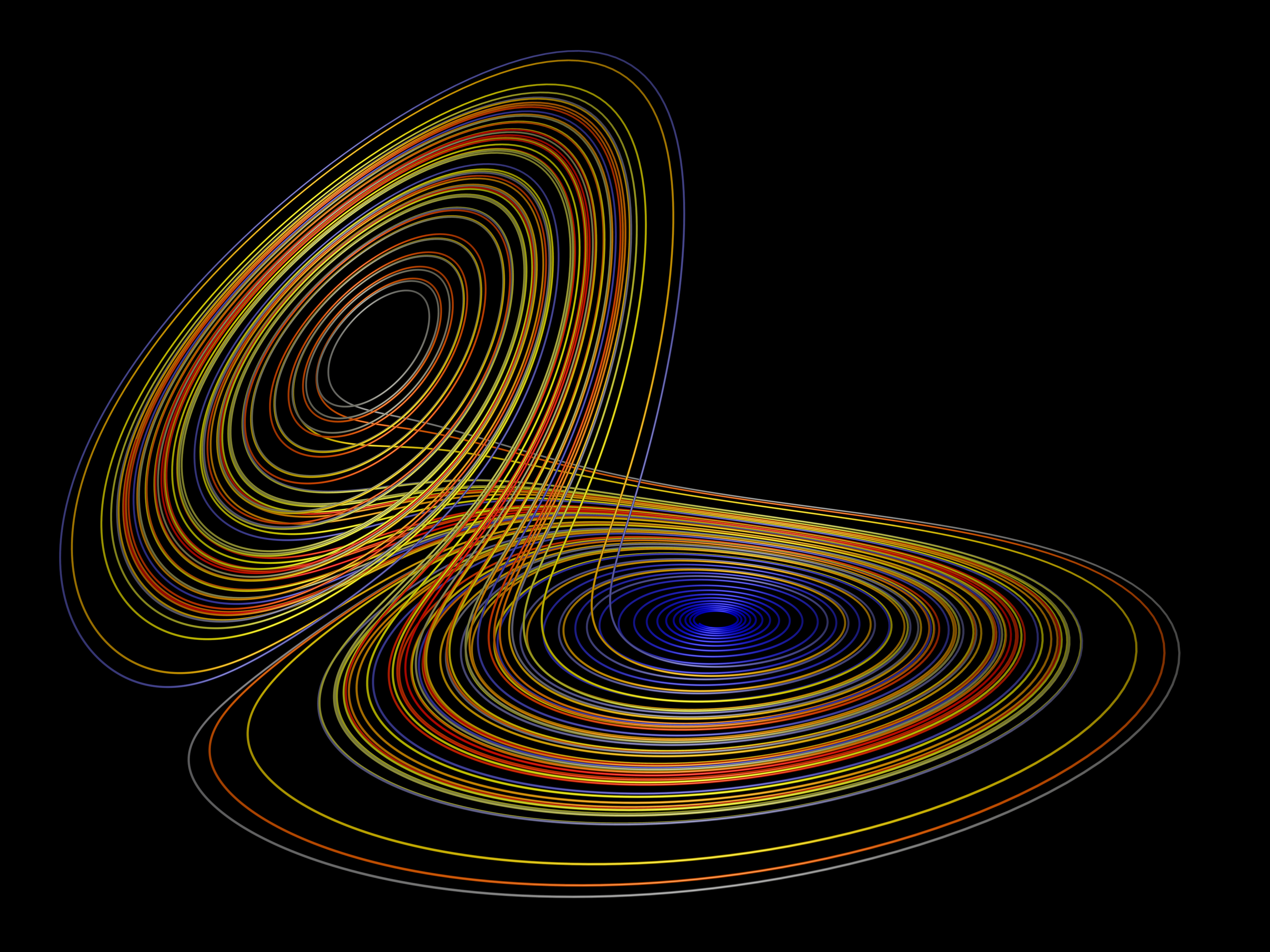
Introduction

In the last post I looked at DMD and EDMD, two methods for analyzing dynamical systems. Both methods look at pairs of snapshots \((x_k, x_{k+1})\) and fit a linear update rule that best predicts the next snapshot. By inspecting that linear map’s eigenvalues and eigenvectors we can learn which patterns dominate and how fast they grow or decay.

Unfortunately, both of these methods rely on a set of features you have chosen in advance. Without the right features you might miss important physics; too many features and the model will become unwieldy. Additionally, while the spectral methods provide some useful insight, they might not have the most easily interpretable output.

What we need is a sparse method, so that we can test a wide number of features and only select the relevant ones for the dynamics, ideally to recover an actual set of interpretable governing equations.

Sparse Identification of Nonlinear Dynamical Systems (SINDy)

SINDy creates a library of candidate basis functions for the eigenfunctions (like EDMD), then does an L1-regularized¹ regression to determine which ones to use. There are two formulations: discrete-time and continuous-time.

Discrete Time

This setup is the same as in DMD and EDMD. We have a discrete-time dynamical system of form:

\[ x_{t+1} = F(x_t) \]

We have our data stream, which we use to create our matrix \(X\):

\[ \mathbf{X} = \begin{bmatrix} \mathbf{x}^T(t_0) \\ \mathbf{x}^T(t_1) \\ \vdots \\ \mathbf{x}^T(t_{m-1}) \end{bmatrix} = \begin{bmatrix} x_1(t_0) & x_2(t_0) & \cdots & x_n(t_0) \\ x_1(t_1) & x_2(t_1) & \cdots & x_n(t_1) \\ \vdots & \vdots & \ddots & \vdots \\ x_1(t_{m-1}) & x_2(t_{m-1}) & \cdots & x_n(t_{m-1}) \end{bmatrix} \]

and its time-shifted counterpart \(Y\):

\[ \mathbf{Y} = \begin{bmatrix} \mathbf{x}^T(t_1) \\ \mathbf{x}^T(t_2) \\ \vdots \\ \mathbf{x}^T(t_m) \end{bmatrix} = \begin{bmatrix} x_1(t_1) & x_2(t_1) & \cdots & x_n(t_1) \\ x_1(t_2) & x_2(t_2) & \cdots & x_n(t_2) \\ \vdots & \vdots & \ddots & \vdots \\ x_1(t_m) & x_2(t_m) & \cdots & x_n(t_m) \end{bmatrix} \]

Now, we need some “library matrix” of relevant basis functions applied to the data (similar to EDMD). This may look something like:

\[ \mathbf{\Theta}(\mathbf{X}) := [\theta_1(X), \theta_2(X),...,\theta_{\ell}(X)] \]

This matrix can be quite large. For example, if the basis functions are drawn from combinations of the monomials \(x_1\), \(x_2\), and \(x_3\) (up to quadratic), we would have something like:

\[ \Theta(X) = \begin{bmatrix} | & | & | & | & | & | & & | \\ 1 & x_1 & x_2 & x_3 & x_1^2 & x_1x_2 & \cdots & x_3^2 \\ | & | & | & | & | & | & & | \end{bmatrix} \]

We are looking for a sparse set of coefficients \(\mathbf{\Xi}\) such that

\[ \mathbf{\Xi} = \begin{bmatrix} | & | & & | \\ \xi_1 & \xi_2 & \cdots & \xi_n \\ | & | & & | \end{bmatrix} \]

This leads us to the SINDy equation:

\[ \mathbf{Y} = \mathbf{\Theta}(\mathbf{X}) \mathbf{\Xi} \]

Each basis function is weighted by a \(\xi_i\). To find the \(\xi_i\), we run a sparse \(L1\)-regularized regression:

\[ \Xi_{opt} = \text{arg }\text{min}_{\Xi} ||\mathbf{Y} - \mathbf{\Theta}(\mathbf{X})\mathbf{\Xi} ||_{2} + \mu||\mathbf{\Xi}||_{1} \]

where \(\mu\) is a parameter controlling the strength of the regularization.

To see the mapping at a single time-step, take the \(k\)-th row of \(\Theta(X)\):

\[ \boxed{\;x^{(k+1)\top} = \Theta\!\bigl(x^{(k)}\bigr)\,\Xi\;}, \quad k=0,\dots,m-1, \]

where

\[ \Theta(x^{(k)})=[\theta_1(x^{(k)}),\dots,\theta_L(x^{(k)})]\in\mathbb R^{1\times L} \]

Continuous Time

A more typical formulation is to assume a dynamical system of the form

\[ \dot{x} = \frac{dx}{dt} = f(x(t)) \]

where \(x\) is the state (possibly a vector) and \(t\) is the time. We have moved from discrete-time to continuous time. We now seek to learn the vector field \(f\), which relates the current state to the rate of change in the state, rather than the next state. Luckily, as we describe in the previous post the Koopman eigenfunctions satisfy:

\[ \frac{d}{dt}\phi(x) = K\phi(x) = \lambda \phi(x) \]

By the chain rule, we also have

\[ \frac{d}{dt}\phi(x) = \nabla \phi(x) \cdot \dot{x} = \nabla \phi(x) \cdot f(x) \]

Combining the two, we have

\[ \nabla \phi(x) \cdot f(x) = \lambda \phi(x) \]

So we can approximate the eigenfunctions via regression². Approximate \(f(x)\) by a sparse weighted sum of dictionary elements:

\[ f(x)\;=\;\sum_{j=1}^{L}\xi_{j}\,\theta_{j}(x)\;=\;\mathbf{\Theta}(x)\,\mathbf{\Xi} \]

This gives:

\[ \nabla\phi(x)\,\cdot\,\mathbf{\Theta}(x)\,\mathbf{\Xi} \;=\;\lambda\,\phi(x) \]

Evaluating at the sample states:

\[ \nabla\phi\!\bigl(\mathbf{x}^{(i)}\bigr)\, \cdot\,\mathbf{\Theta}\!\bigl(\mathbf{x}^{(i)}\bigr)\, \mathbf{\Xi} \;=\; \lambda\, \phi\!\bigl(\mathbf{x}^{(i)}\bigr), \quad i=1,\dots,m \]

Now we have

\[ \mathbf{\dot X} \;=\; \mathbf{\Theta}(\mathbf{X})\,\mathbf{\Xi}, % (5) \quad\text{where} \; \mathbf{\dot X} = \begin{bmatrix} \dot{\mathbf x}^{(1)\!\top}\\ \dot{\mathbf x}^{(2)\!\top}\\ \vdots\\ \dot{\mathbf x}^{(m)\!\top} \end{bmatrix},\; \mathbf{\Theta}(\mathbf{X}) = \begin{bmatrix} \mathbf{\Theta}(x^{(1)})\\ \mathbf{\Theta}(x^{(2)})\\ \vdots\\ \mathbf{\Theta}(x^{(m)}) \end{bmatrix} \]

and so we can solve the continuous-time problem with the following regression

\[ \mathbf{\Xi}_{opt} \;=\; \operatorname*{arg\,min}_{\mathbf{\Xi}} \Bigl\| \mathbf{\dot X} - \mathbf{\Theta}(\mathbf{X})\,\mathbf{\Xi} \Bigr\|_{2} \;+\; \mu\,\|\mathbf{\Xi}\|_{1} \]

Conveniently, exactly the same as the previous regression equation, except here we are approximating:

\[ \frac{dx}{dt} = f(x(t)) = \mathbf{\Theta}(x)\mathbf{\Xi} \]

Implementation

To implement SINDy, we need a library matrix function and a method of handling the regression. We may also want a finite differences method, to calculate derivatives.

Finite Differences

We will use finite differences³ to approximate the time derivative by dividing small state increments by the timestep \(\Delta t\).

At an interior point \(t_i\) we use the second-order central stencil
\[ \dot x(t_i)\;\approx\;\frac{x(t_{i+1}) - x(t_{i-1})}{2\,\Delta t}, \]

which cancels the first-order truncation error, yielding \(\mathcal{O}(\Delta t^{2})\) accuracy.

At the boundaries we fall back to the first-order forward and backward stencils: \[ \dot x(t_0)\;\approx\;\frac{x(t_1)-x(t_0)}{\Delta t}, \qquad \dot x(t_{m-1})\;\approx\;\frac{x(t_{m-1})-x(t_{m-2})}{\Delta t}. \]

def finite_difference(X, dt):
    n_vars, n_samples = X.shape
    
    # Use central differences where possible, forward/backward at boundaries
    dXdt = np.zeros((n_samples, n_vars))
    
    # Forward difference at first point
    dXdt[0, :] = (X[:, 1] - X[:, 0]) / dt
    
    # Central differences for interior points
    for i in range(1, n_samples - 1):
        dXdt[i, :] = (X[:, i + 1] - X[:, i - 1]) / (2 * dt)
    
    # Backward difference at last point
    dXdt[-1, :] = (X[:, -1] - X[:, -2]) / dt
    
    return dXdt

The helper above implements exactly this scheme: it accepts a state matrix of shape \((n_{\text{vars}}, n_{\text{samples}})\), returns the derivative matrix \((n_{\text{samples}}, n_{\text{vars}})\), and also transposes \(X\) so rows correspond to time snapshots for the subsequent regression.

Library Matrix

Next we build the candidate feature matrix \(\Theta\) by stacking a constant term, all monomials up to poly_order, and optionally sine/cosine transforms of each state variable. Returns that matrix along with a parallel descriptions list so the sparse coefficients can later be mapped back to human-readable terms.

def sindy_library(X, poly_order=3, include_sine=False, include_cosine=False):
    n_vars, n_samples = X.shape
    
    # Start with constant term
    library_functions = [np.ones(n_samples)]
    descriptions = ['1']
    
    # Add polynomial terms
    for order in range(1, poly_order + 1):
        for combo in combinations_with_replacement(range(n_vars), order):
            if order == 1:
                var_idx = combo[0]
                library_functions.append(X[var_idx, :])
                descriptions.append(f'x_{var_idx}')
            else:
                term = np.ones(n_samples)
                term_desc = []
                for var_idx in combo:
                    term *= X[var_idx, :]
                    term_desc.append(f'x_{var_idx}')
                library_functions.append(term)
                descriptions.append('*'.join(term_desc))
    
    # Add trigonometric terms if requested
    if include_sine:
        for i in range(n_vars):
            library_functions.append(np.sin(X[i, :]))
            descriptions.append(f'sin(x_{i})')
            
    if include_cosine:
        for i in range(n_vars):
            library_functions.append(np.cos(X[i, :]))
            descriptions.append(f'cos(x_{i})')
    
    Theta = np.column_stack(library_functions)
    
    return Theta, descriptions

Sequential Threshold Least Squares

We will use Sequential Threshold Least Squares to obtain the full coefficient matrix.

At each iteration \(k\):

Set every entry with \(|\xi_{ij}^{(k)}| < \lambda_{reg}\) to zero, forcing small terms out of the model⁴.
Refit for each state component \(j\), solve a new least–squares problem using only the surviving (non-zero) columns of \(\Theta\) to get updated weights.
Repeat until convergence or for at most max_itercycles; the final \(\Xi\) contains only the terms that remain large after repeated shrink-and-refit, giving a sparse governing equation.

def sequential_threshold_least_squares(Theta, dXdt, lambda_reg=0.1, max_iter=10):
    n_states = dXdt.shape[1]
    
    # Initialize coefficient matrix
    Xi = np.linalg.lstsq(Theta, dXdt, rcond=None)[0]
    
    # Iterative thresholding
    for iteration in range(max_iter):

        # Find small coefficients to remove
        small_inds = np.abs(Xi) < lambda_reg
        
        # Set small coefficients to zero
        Xi[small_inds] = 0
        
        # Identify active (non-zero) coefficients for each state
        for i in range(n_states):
            big_inds = ~small_inds[:, i]
            if np.any(big_inds):
                
                # Recompute non-zero coefficients using least squares
                Xi[big_inds, i] = np.linalg.lstsq(
                    Theta[:, big_inds], dXdt[:, i], rcond=None
                )[0]
            else:
                Xi[:, i] = 0
    
    return Xi

`print_equations`

I’ll add one bonus helper function, which will be useful later

def print_equations(Xi, descriptions, feature_names=None):
    n_functions, n_features = Xi.shape
    
    if feature_names is None:
        feature_names = [f'x_{i}' for i in range(n_features)]
        
    for i in range(n_features):

        # Build equation string
        terms = []
        for j in range(n_functions):
            coef = Xi[j, i]
            if abs(coef) > 1e-10:  # Only include non-zero terms
                if abs(coef - 1.0) < 1e-10:
                    terms.append(f"{descriptions[j]}")
                elif abs(coef + 1.0) < 1e-10:
                    terms.append(f"-{descriptions[j]}")
                else:
                    terms.append(f"{coef:.6f}*{descriptions[j]}")
        
        if terms:
            equation = " + ".join(terms).replace(" + -", " - ")
            print(f"d{feature_names[i]}/dt = {equation}")
        else:
            print(f"d{feature_names[i]}/dt = 0")
    print()

Integration

Putting the piece together:

def sindy(X, dXdt, poly_order=3, lambda_reg=0.1, include_sine=False, 
          include_cosine=False, max_iter=10):
    
    # Build library of candidate functions
    Theta, descriptions = sindy_library(
        X, 
        poly_order=poly_order, 
        include_sine=include_sine, 
        include_cosine=include_cosine
    )
    
    # Sparse regression using sequential thresholded least squares
    Xi = sequential_threshold_least_squares(Theta, dXdt, lambda_reg, max_iter)
    
    return Xi, descriptions

For a production version you may want to factor the library production out of the SINDy method.

Experiments

Let’s generate data from few known systems and see if SINDy can recover their governing equations.

Simple Harmonic Oscillator

Definition

The simple harmonic oscillator is described by the following second-order ODE:

\[ x'' + \omega^2 x = 0 \]

If we let: \[ \begin{align} x_0 &:= x \\ x_1 &:= \frac{dx}{dt} \end{align} \]

We can then derive

\[ \begin{align} \frac{dx_0}{dt} &= \frac{dx}{dt} = x_1 \\ \frac{dx_1}{dt} &= - \omega^2 x_0 \end{align} \]

So it has an alternative formulation as a set of coupled first-order ODEs.

Approximation

The simple harmonic oscillator has a well-known analytic solution: \[ x = \cos(\omega t) \]

Let

def generate_simple_harmonic_oscillator_data(omega=2.0, t_final=10, dt=0.01):
    t = np.arange(0, t_final, dt)
    
    # Analytical solution
    x = np.cos(omega * t)
    xdot = -omega * np.sin(omega * t)
    
    X_train = np.vstack([x, xdot])
    
    return X_train

This will give us data for the harmonic oscillator⁵.

Now we run SINDy on this data:

X = generate_simple_harmonic_oscillator_data()
dXdt = finite_difference(X, dt)                
Xi, desc = sindy(X, dXdt, poly_order=1, lambda_reg=0.1)
print_equations(Xi, desc, feature_names=['x_0', 'x_1'])

We discover the following equations:

dx_0/dt = 0.999925*x_1
dx_1/dt = -3.999764*x_0

Which is close to the true generating equations:

\[ \begin{align} \frac{dx_0}{dt} &= x_1 \\ \frac{dx_1}{dt} &= -4 x_0 \end{align} \]

Lorenz System

Definition

The Lorenz-63 model is a three-dimensional ODE derived from a truncated Fourier expansion of the Boussinesq equations for thermal convection. In its nondimensional form the state \(\mathbf{x}=(x,y,z)^{\!\top}\) evolves as

\[ \begin{aligned} \dot x &= \sigma \,(y - x), \\ \dot y &= x \,(\rho - z) - y, \\ \dot z &= x\,y - \beta\,z, \end{aligned} \]

Let us recover this equation from data.

Approximation

def generate_lorenz_data(initial_conditions, sigma=10, rho=28, beta=8/3, t_final=10, dt=0.01):
    
    def lorenz_rhs(state, sigma=sigma, rho=rho, beta=beta):
        x, y, z = state
        return np.array([
            sigma * (y - x),
            x * (rho - z) - y,
            x * y - beta * z
        ])
    
    # Generate training data
    t_train = np.arange(0, t_final, dt)
    n_steps = len(t_train)
    
    X_train = np.zeros((3, n_steps))
    X_train[:, 0] = initial_conditions 
    
    for i in range(1, n_steps):
        k1 = lorenz_rhs(X_train[:, i-1])
        k2 = lorenz_rhs(X_train[:, i-1] + dt/2 * k1)
        k3 = lorenz_rhs(X_train[:, i-1] + dt/2 * k2)
        k4 = lorenz_rhs(X_train[:, i-1] + dt * k3)
        X_train[:, i] = X_train[:, i-1] + dt/6 * (k1 + 2*k2 + 2*k3 + k4)

    return X_train

Following the same steps:

initial_conditions = [-8, 8, 27] 
X = generate_lorenz_data(initial_conditions)

dXdt = finite_difference(X, dt)                
Xi, desc = sindy(X, dXdt, poly_order=2, lambda_reg=0.05)

print_equations(Xi, desc, feature_names=['x', 'y', 'z'])

We discover the following equations:

dx/dt = -9.971816*x_0 + 9.972789*x_1
dy/dt = 27.823397*x_0 - 0.970096*x_1 - 0.994849*x_0*x_2
dz/dt = -2.658203*x_2 + 0.996862*x_0*x_1

Which is once again pretty close to the actual generating equations (rewritten): \[ \begin{align} \frac{dx_0}{dt} &= -10x_0 + 10x_1 \\ \frac{dx_1}{dt} &= 28x_0 - x_1 - x_0x_2 \\ \frac{dx_2}{dt} &= -\frac{8}{3}x_2 + x_0x_1 \end{align} \]

Conclusion

We used SINDy to recover governing equations for two toy problems.

SINDy Method for Learning Dynamical Systems

Introduction

Sparse Identification of Nonlinear Dynamical Systems (SINDy)

Discrete Time

Continuous Time

Implementation

Finite Differences

Library Matrix

Sequential Threshold Least Squares

`print_equations`

Integration

Experiments

Simple Harmonic Oscillator

Definition

Approximation

Lorenz System

Definition

Approximation

Conclusion

Further Reading

Footnotes