Introduction
In the dynamical similarity post we looked at equivariant symmetries of the Lagrangian, which produce Noether-like quantities that are conserved not within a single trajectory but across families of similar trajectories. That is, given \(g \in G\):
\[ L(\Phi_g(q), T\Phi_g(\dot q)) = \chi(g) \cdot L(q, \dot q) \]
where \(\chi: G \to \mathbb{R}_{>0}\) is a group homomorphism. In particular, Kepler’s third law fell out as a special case. The scaling symmetry \((t, q) \mapsto (\lambda^\alpha t, \lambda q)\) with \(\alpha = 3/2\) gives the relationship between orbital radius and period.
In the invariant theory work we used computational invariant theory to study games. This followed a similar pattern of applying some group homomorphism to an underlying representation, and then using the invariants to classify the actual objects into equivalence classes.
Similar ideas exist with respect to the biological concept of allometry. In biology, allometry is the study of how biological traits scale with body size, usually through power laws such as metabolic rate scaling as mass to the \(3/4\)-power, known as Kleiber’s law. The modern quarter-power scaling story is also associated with the fractal network model of West, Brown, and Enquist, and with later attempts to extend allometric scaling from genomes to ecosystems. However, the same scaling concepts have also been applied outside organismal biology, including to the scaling of cities.
While allometry is usually seen as a set of empirical power laws, in this post I will attempt to ground it at least partially in invariant theory, and show that the typical allometric setup is the \(\mathrm{GL}(1)\) instance of the invariant-theoretic scaling framework we’ve already been using (and therefore our invariant theory framework can be seen as generalizing allometry). Based on this, when we see an empirical relationship, we ought to be able to infer the type of constraint that’s governing the set of possible forms1.
1 We can still think of this as an empirical method if we want: given a generator, predict invariant combinations and compute residuals. I mostly don’t do that here, to present the framework.
Allometric Scaling Laws
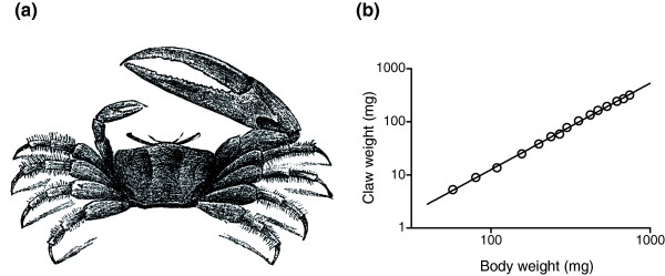
The claw of the fiddler crab grows faster than its body. A small crab has a modest claw, but a large crab has an outsized one. In his 1932 book Problems of Relative Growth, Huxley showed that the size of the claw scales as roughly \(M^{1.6}\) (where \(M\) is the crab’s body mass). This is a typical allometric relation, where a trait scales as a power law of some underlying body size dimension of the organism.
Let’s attempt to rederive the power law structure via algebraic means.
Let \(M\) denote body mass. More generally, we can assume a single dimension parametrizing the size or scale of the system, and call it \(M\), but for the sake of this discussion we will assume \(M\) is the mass. Therefore, all the other biological traits will be compared with respect to \(M\). In that vein, let \(Y(M)\) denote some trait as a function of body mass, such as metabolic rate, heart rate, lifespan, organ volume, transport distances, or some other morphological measurement.
A biological system is described by a collection of these coupled variables. A change in body mass moves the system through this larger trait space. However, even though larger systems may require different transport distances, rates, energetic throughputs, organ sizes, and characteristic times, we assume that (to remain the same system type), the quantities must still fit together in a similar way to the smaller system version to remain functional.
Therefore, we assume that changing body mass by a factor \(\lambda\) induces a coordinated change in each associated trait, and the induced change depends on the factor \(\lambda\) rather than on the path used to get there. For a single trait \(Y\), this means there is a response function \(A\) such that
\[ Y(\lambda M) = A(\lambda)Y(M) \]
The function \(A(\lambda)\) records how the trait responds to a size-rescaling by \(\lambda\).
Mathematically, this means that body-size rescaling is represented by a one-parameter action on the full trait vector. If \(M\) is body mass and \(\mathbf{x} = (x_1,\ldots,x_n)\) records the other traits, then a rescaling by \(\lambda > 0\) acts as
\[ (M, x_1,\ldots,x_n) \mapsto (\lambda M, A_1(\lambda)x_1,\ldots,A_n(\lambda)x_n) \]
Also, scaling first by \(\mu\) and then by \(\lambda\) is the same scaling of mass as scaling once by \(\lambda\mu\), so the associated trait response must compose in the same way:
\[ A(\lambda\mu) = A(\lambda)A(\mu) \]
Assume \(A\) is positive and continuous. Define
\[ a(t)=\log A(e^t) \]
Then
\[ a(t+s) = \log A(e^{t+s}) = \log A(e^t e^s) = \log(A(e^t)A(e^s)) = a(t)+a(s) \]
So \(a\) satisfies the additive Cauchy equation. Since \(a\) is continuous, there is some \(\alpha \in \mathbb{R}\) such that
\[ a(t)=\alpha t \]
Therefore
\[ \log A(e^t)=\alpha t \]
so
\[ A(e^t)=e^{\alpha t} \]
Writing \(\lambda=e^t\), we get
\[ A(\lambda)=\lambda^\alpha \]
Substituting this back into the scaling equation gives
\[ Y(\lambda M)=\lambda^\alpha Y(M) \]
Now fix a reference mass \(M_0\) and take \(\lambda=M/M_0\). Then, for any body mass \(M>0\),
\[ Y(M)=Y\!\left(\frac{M}{M_0}\,M_0\right)=\left(\frac{M}{M_0}\right)^\alpha Y(M_0). \]
Writing \(k=Y(M_0)\,M_0^{-\alpha}\) recovers the usual form \(Y=kM^\alpha\).
Thus the allometric power law is the unique continuous solution to the compositional scaling assumption.
Across the full set \[ (M, x_1,\ldots,x_n) \mapsto (\lambda M, A_1(\lambda)x_1,\ldots,A_n(\lambda)x_n) \]
Across the full set of traits, the same assumption says that body-size rescaling acts diagonally on trait space:
\[ (M, x_1,\ldots,x_n) \mapsto (\lambda M, A_1(\lambda)x_1,\ldots,A_n(\lambda)x_n) \]
We can thus say that each trait carries a one-dimensional response representation of the scaling group \(\mathbb{R}_{>0}\). Compositional consistency forces each response function \(A_i\) to satisfy
\[ A_i(\lambda\mu)=A_i(\lambda)A_i(\mu) \]
Assuming each \(A_i\) is positive and continuous, the same Cauchy-equation argument gives
\[ A_i(\lambda)=\lambda^{w_i} \]
for some weight \(w_i \in \mathbb{R}\). Therefore the full scaling action becomes
\[ (M, x_1,\ldots,x_n) \mapsto (\lambda M, \lambda^{w_1}x_1,\ldots,\lambda^{w_n}x_n) \]
The numbers \(w_i\) are the allometric weights of the traits relative to body mass.
Invariant-Theoretic Interpretation
This is now an invariant-theory problem. We have a group, the positive component of \(\mathrm{GL}(1,\mathbb{R})\),
\[ G = \mathbb{R}_{>0}, \]
acting on a positive trait space with coordinates \((M,x_1,\ldots,x_n)\):
\[ \lambda \cdot (M,x_1,\ldots,x_n) = (\lambda M,\lambda^{w_1}x_1,\ldots,\lambda^{w_n}x_n) \]
Body mass has weight \(1\), and trait \(x_i\) has weight \(w_i\). A monomial in these variables has the form
\[ I_{\beta} (M,\mathbf{x}) = M^{\beta_0}\prod_{i=1}^n x_i^{\beta_i} \]
Under the scaling action, it transforms as
\[ I_{\beta}(\lambda M,\lambda^{w_1}x_1,\ldots,\lambda^{w_n}x_n) = \lambda^{\beta_0 + \sum_i w_i\beta_i} I_{\beta}(M,\mathbf{x}) \]
Therefore \(I_{\beta}\) is invariant exactly when the total weight vanishes:
\[ \beta_0 + \sum_i w_i\beta_i = 0 \]
Equivalently, if the rank-one weight matrix is
\[ W = \begin{pmatrix} 1 & w_1 & \cdots & w_n \end{pmatrix} \]
then the invariant monomials are exactly those whose exponent vectors lie in the kernel:
\[ W\beta = 0 \]
On the positive cone the exponents may be real, so these are generalized monomial invariants. When the weights are rational and the exponents integral after clearing denominators, they recover the usual algebraic torus invariant ring.
For a single trait \(Y\) with weight \(\alpha\), the invariant condition is
\[ \beta_M + \alpha \beta_Y = 0 \]
Taking \(\beta_Y = 1\) gives \(\beta_M = -\alpha\), hence the invariant
\[ I(M,Y)=YM^{-\alpha} \]
Setting this invariant equal to a constant gives
\[ YM^{-\alpha}=k \]
or
\[ Y=kM^\alpha \]
So the usual allometric law is the invariant of the \(\mathrm{GL}(1)\) scaling action written back in the original coordinates. The regression line on a log-log plot is the shadow of an invariant monomial.
Alternatively, we can read the same algebra covariantly. The scaling action assigns each coordinate a character of \(\mathrm{GL}(1)\). Body mass transforms with character \(\lambda\):
\[ M \mapsto \lambda M \]
and a trait \(Y\) with allometric weight \(\alpha\) transforms with character \(\lambda^\alpha\):
\[ Y \mapsto \lambda^\alpha Y \]
This says that \(Y\) is a covariant of weight \(\alpha\). The quantity \(M^\alpha\) is also a covariant of weight \(\alpha\), since
\[ M^\alpha \mapsto (\lambda M)^\alpha = \lambda^\alpha M^\alpha \]
Thus \(Y\) and \(M^\alpha\) live in the same one-dimensional representation of the scaling group. The allometric law says that these two covariants are proportional:
\[ Y = kM^\alpha \]
The invariant formulation is obtained by canceling the common character:
\[ \frac{Y}{M^\alpha} \mapsto \frac{\lambda^\alpha Y}{\lambda^\alpha M^\alpha} = \frac{Y}{M^\alpha} \]
So the invariant \(YM^{-\alpha}\) is the quotient of two covariants with the same weight.
This gives the equivalence-class interpretation. Represent an organism by its point in trait space,
\[ p = (M,x_1,\ldots,x_n) \in \mathbb{R}_{>0}^{n+1} \]
The scaling action sends this point to
\[ \lambda \cdot p = (\lambda M,\lambda^{w_1}x_1,\ldots,\lambda^{w_n}x_n) \]
Two organisms \(p\) and \(p'\) are allometrically equivalent, relative to the chosen weights \(W\), when one can be obtained from the other by such a rescaling:
\[ p' \sim_W p \quad \Longleftrightarrow \quad p' = \lambda \cdot p \text{ for some } \lambda \in \mathbb{R}_{>0} \]
The equivalence class of \(p\) is its scaling orbit,
\[ [p]_W = \{\lambda \cdot p : \lambda \in \mathbb{R}_{>0}\} \]
Along this orbit, the raw trait values change covariantly, while the invariant monomials stay fixed. Thus the quotient
\[ \mathbb{R}_{>0}^{n+1}/\mathbb{R}_{>0} \]
is the space of allometric types, and organisms are identified when they differ only by the coordinated size-rescaling prescribed by the weights.
In the single-trait case, the invariant
\[ YM^{-\alpha} \]
labels the orbit. Two organisms with trait-mass pairs \((M,Y)\) and \((M',Y')\) lie in the same allometric equivalence class exactly when
\[ YM^{-\alpha}=Y'(M')^{-\alpha} \]
Equivalently, they share the same allometric constant \(k\).2 In the one-trait case, each level set of the invariant is a scaling orbit. In the multi-trait case, the full collection of invariant monomials gives the quotient coordinates that classify the scaling orbits.
2 Biologists call groups that share an exponent but differ in \(k\) grades (e.g. endotherms vs. ectotherms), so grades are just different orbits.
Relationship to the Buckingham \(\pi\) Theorem
The Buckingham \(\pi\) theorem is the same idea in the language of dimensional analysis.
Suppose we have \(n\) positive quantities
\[ \mathbf{x}=(x_1,\ldots,x_n) \]
and \(k\) independent base scales (note that this is a slightly different setup than before, as we have multiple scaling axes). These base scales may be physical dimensions such as mass, length, and time, or they may be biological scaling axes chosen for the model. The scaling group is the torus
\[ G=(\mathbb{R}_{>0})^k \]
Each coordinate \(x_i\) has a weight vector recording how it transforms under the \(k\) base scales. Put these weights into a matrix
\[ W \in \mathbb{Q}^{k \times n} \]
If \(g=(g_1,\ldots,g_k)\in G\), then the action is
\[ x_i \mapsto \prod_{r=1}^k g_r^{W_{ri}}x_i \]
A monomial
\[ \Pi_\beta(\mathbf{x})=\prod_{i=1}^n x_i^{\beta_i} \]
is invariant exactly when its total weight vanishes:
\[ W\beta=0 \]
These invariant monomials are the Buckingham \(\pi\) groups, which are the dimensionless coordinates on the quotient space
\[ \mathbf{X}/G \]
So Buckingham \(\pi\) can be thought of as a quotient construction. We start with the full coordinate space of measured quantities, divide by the scaling action of the base dimensions, and use invariant monomials as coordinates on the reduced space.
In the rank-one allometric case, the weight matrix is
\[ W= \begin{pmatrix} 1 & \alpha \end{pmatrix} \]
for the coordinates \((M,Y)\). The kernel condition
\[ W\beta=0 \]
is
\[ \beta_M+\alpha\beta_Y=0 \]
Taking \(\beta_Y=1\) gives the invariant
\[ \Pi = YM^{-\alpha} \]
So the single-trait case is the one-dimensional Buckingham \(\pi\) construction, and the allometric constant is the quotient coordinate.
For multiple traits, the same construction produces all independent dimensionless combinations admitted by the chosen weights. If
\[ W= \begin{pmatrix} 1 & w_1 & \cdots & w_n \end{pmatrix}, \]
then the \(\pi\) groups are all monomials
\[ \Pi_\beta(M,\mathbf{x})=M^{\beta_0}\prod_i x_i^{\beta_i} \]
with
\[ \beta_0+\sum_i w_i\beta_i=0 \]
In other words, the Buckingham \(\pi\) theorem is the invariant-theoretic statement that the quotient by a torus action is coordinatized by monomial invariants, which we have seen before.
A familiar non-biological example is the Reynolds number. Take the variables
\[ (\rho, v, L, \mu) \]
where \(\rho\) is density, \(v\) is velocity, \(L\) is length, and \(\mu\) is dynamic viscosity. Changes of unit are multiplicative and independently selectable across the base dimensions. If the base dimensions are mass, length, and time, then a change of units is specified by
\[ g=(g_M,g_L,g_T)\in(\mathbb{R}_{>0})^3 \]
Each measured quantity transforms covariantly according to its dimensions. In base dimensions \((M,L,T)\), their weights are
\[ [\rho] = M L^{-3}, \qquad [v] = L T^{-1}, \qquad [L] = L, \qquad [\mu] = M L^{-1}T^{-1} \]
So the weight matrix is
\[ W = \begin{pmatrix} 1 & 0 & 0 & 1 \\ -3 & 1 & 1 & -1 \\ 0 & -1 & 0 & -1 \end{pmatrix} \]
A monomial
\[ \Pi = \rho^{\beta_\rho}v^{\beta_v}L^{\beta_L}\mu^{\beta_\mu} \]
is dimensionless when
\[ W\beta=0 \]
One kernel vector is
\[ \beta = (1,1,1,-1) \]
which gives
\[ \Pi = \frac{\rho v L}{\mu} \]
which is the Reynolds number. So two fluid flow systems are similar if they have the same Reynolds number.
In the language of the reduction post, the quotient removes directions generated by the group action. This is especially useful for control tasks because those directions are structurally predictable, as they come from symmetry rather than from the task-relevant dynamics. Designing feedback on the quotient space focuses a controller on the reduced state, where symmetry-related configurations have already been identified.
Buckingham \(\pi\) gives the scaling version of the same idea. The raw variables include directions corresponding to arbitrary choices of base scale; the \(\pi\) groups are the reduced coordinates. Controlling or comparing systems through the \(\pi\) groups means acting on the similarity class directly, rather than on a particular representative of that class.
Generalized Allometries
Transformation and Generated Families

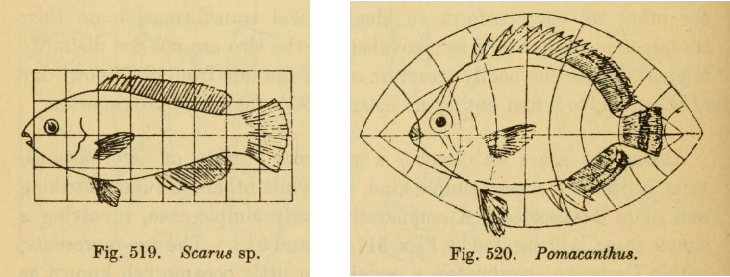
In On Growth and Form, Darcy Thompson compares animal forms by drawing one organism on a coordinate grid and then deforming the grid so that the transformed coordinates change one fish species into another.
A biological form is represented in some space of coordinates, and a transformation acts on that space. The orbit of the transformation is the family of forms produced by varying the transformation parameter3. If we quotient out this transformation, we can get an equivalence class of possible forms.
3 Note the likely restrictions here. The full range of transformations is probably not available due to external constraints. More on this later.
In standard allometry, we peg everything to body size, and a trait vector moves along a scaling orbit, such as
\[ (M,x_1,\ldots,x_n) \mapsto (\lambda M,\lambda^{w_1}x_1,\ldots,\lambda^{w_n}x_n) \]
But Thompson’s grids suggest broader possibilities. Instead of only considering forms under scaling by \(GL(1)\), the generator may be a more deformation of the coordinate system in which the organism is represented. Size is then just one possible generator, as we could potentially also apply stretching, shears, rotations, or other transformations to generate structured families of biological forms.
Let \(Q\) be the space in which a form is represented, and let \(S \subset Q\) be a biological form, such as an outline, a landmark configuration, a surface, or a point cloud.
Assume that comparisons across a family must compose. For example, if \(q_a\) is compared to \(q_b\) by \(g_{ba}\), and \(q_b\) is compared to \(q_c\) by \(g_{cb}\), then the direct comparison from \(q_a\) to \(q_c\) is
\[ g_{ca}=g_{cb}g_{ba} \]
If we also assume that there is an identity transformation, then we are essentially assuming that a group \(G\) acts on \(Q\), and therefore acts on forms by
\[ S \mapsto g\cdot S \]
The orbit of \(S\) is
\[ G\cdot S = \{g\cdot S : g\in G\} \]
This orbit is the family of forms generated by the chosen transformation, and the quotient \(Q/G\) is the reduced space in which forms related by that transformation are compared through the same coordinates.
For ordinary allometry, composition is just multiplication of body-mass ratios. If
\[ \lambda_{ba}=\frac{M_b}{M_a} \]
then
\[ \lambda_{ca} = \frac{M_c}{M_a} = \frac{M_c}{M_b}\frac{M_b}{M_a} = \lambda_{cb}\lambda_{ba} \]
The covariants describe how the measured quantities change across the family. The invariants are the reduced coordinates that don’t change under transformation:
\[ I(g\cdot q)=I(q) \]
Note: This is speculative, but why should the forms lie along the orbits of a group? First of all, clearly we are not talking about full groups, but rather semigroups or local groups. Imagine stretching a fish until it is completely flat, like a line - obviously that won’t work as the fish will die. Even if a mathematical transformation family exists, the biologically admissible parameter range is bounded away from singular, nonviable, or mechanically impossible regimes. But I would conjecture that, under some process of optimization, forms tend to the limits of their constraints (they cannot optimize beyond the constraints, as the form would be non-viable). Since symmetries and groups are deeply involved in physics (more on this in a future post), we end up with these group-like constraints on evolutionary or ontogenic forms. So forms lie near group-like orbits because biological variation is generated by composable processes, and selection filters the viable region of those generated possibilities.
Furthermore, what happens when the group acting on the space of forms is something other than \(GL(1)\)? In this case we will have a similar algebraic framework to standard allometry, but generalized to accomodate different symmetries.
Coupled Scaling
The textbook allometric example compares metabolic rate to body mass:

Note that the curve is not quite a straight line. On log-log axes the exponent drifts over the range of sizes sampled.
The toric generator we assumed in the previous section assumed that each trait scaled independently as we increased the size. However, it’s possible for two traits to scale together rather than independently. Coupling shows up algebraically as a scaling generator that cannot be diagonalized, and a non-diagonalizable generator bends a clean power law into a power law with a logarithmic correction.
Let’s look at this mathematically. Ordinary allometry used a scalar response:
\[ Y(\lambda M)=A(\lambda)Y(M) \]
For coupled traits, the response is matrix-valued instead:
\[ \mathbf{Y}(\lambda M)=A(\lambda)\mathbf{Y}(M), \qquad A(\lambda)\in\mathrm{GL}(2,\mathbb{R}) \]
Composition is the same as before:
\[ A(\lambda\mu)=A(\lambda)A(\mu) \]
Writing
\[ \tilde A(t)=A(e^t) \]
we get a one-parameter subgroup of \(\mathrm{GL}(2,\mathbb R)\):
\[ \tilde A(t)=e^{tX} \]
for a fixed generator \(X\).
If \(X\) is diagonalizable, a change of basis decouples the traits into independent power laws, which was the case we had before. However, what if the matrix is non-diagonalizable? Then the degenerate limit is nilpotent \(X=\begin{pmatrix}0&1\\0&0\end{pmatrix}\), which adds one coordinate to another with no scaling and thus no power law. The allometric case keeps a common eigenvalue \(w\), giving the Jordan block:
\[ X= \begin{pmatrix} w&1\\ 0&w \end{pmatrix} \]
Then, with \(t=\log\lambda\),
\[ e^{tX} = \lambda^w \begin{pmatrix} 1&\log\lambda\\ 0&1 \end{pmatrix} \]
Composition still holds, since \(e^{tX}e^{sX}=e^{(t+s)X}\) and the unipotent parts simply add:
\[ \begin{pmatrix} 1&\log\lambda\\ 0&1 \end{pmatrix} \begin{pmatrix} 1&\log\mu\\ 0&1 \end{pmatrix} = \begin{pmatrix} 1&\log\lambda+\log\mu\\ 0&1 \end{pmatrix} \]
Componentwise,
\[ Y_2(\lambda M)=\lambda^wY_2(M) \]
and
\[ Y_1(\lambda M)=\lambda^w\left(Y_1(M)+(\log\lambda)Y_2(M)\right) \]
The second trait is an ordinary power law:
\[ Y_2(M)=k_2M^w \]
For \(Y_1\), write
\[ Y_1(M)=M^wf(\log M) \]
Then the scaling equation becomes
\[ f(u+t)=f(u)+k_2t \]
where
\[ u=\log M, \qquad t=\log\lambda \]
Thus
\[ f(u)=k_1+k_2u \]
(after choosing a reference scale). Writing the logarithm dimensionlessly with \(M_0\),
\[ Y_1(M)=M^w\left(k_1+k_2\log(M/M_0)\right) \]
while
\[ Y_2(M)=k_2M^w \]
So a Jordan block gives a power law with a logarithmic correction.
If we keep adding coupled variables, the same pattern continues. A size-\(r\) Jordan block has the form
\[ X=wI+C \]
where
\[ C= \begin{pmatrix} 0&1&0&\cdots&0\\ 0&0&1&\cdots&0\\ \vdots&\vdots&\ddots&\ddots&1\\ 0&0&\cdots&0&0 \end{pmatrix} \]
and \(C^r=0\). Therefore
\[ e^{tX} = e^{tw} \sum_{m=0}^{r-1}\frac{t^m}{m!}C^m \]
With \(t=\log\lambda\), this becomes
\[ \lambda^X = \lambda^w \sum_{m=0}^{r-1} \frac{(\log\lambda)^m}{m!}C^m \]
So a Jordan block produces one shared power law multiplied by a polynomial in \(\log M\).
Choosing a reference scale \(M_0\) and writing
\[ \ell=\log(M/M_0) \]
the solutions are
\[ Y_i(M) = M^w \sum_{j=i}^{r} k_j \frac{\ell^{j-i}}{(j-i)!} \]
For example, with three coupled variables,
\[ Y_3(M)=k_3M^w \]
\[ Y_2(M)=M^w(k_2+k_3\ell) \]
and
\[ Y_1(M) = M^w \left( k_1+k_2\ell+\frac12k_3\ell^2 \right) \]
Interestingly, if we look at work on metabolic scaling rate in mammals (such as Kolokotrones et al. 2010) we see that the authors propose similar rules for fitting the curves.
The algebraic framework gives us a structural hypothesis to go along with the empirical scaling law. We ought to see these types of log-polynomial rules if the underlying scaling mechanism has repeated modes that are coupled rather than independently diagonalizable. In that case, curvature on the log-log plot may indicate that one normalized trait drives the log-size drift of another.
Biologically, this would mean the bend is produced by two physiological quantities that share the same baseline scaling law, but are coupled so that each multiplicative increase in body size adds a fixed amount of one normalized quantity into the other. In other words, every octave of body mass would push the system a little farther along the same coupled allocation/transport/metabolic mode.
So (speculatively) the mechanism should look like a same-exponent feed-forward relation. After removing the common \(M^w\) scaling, one trait remains approximately constant while the other accumulates in proportion to it. For metabolism, that would suggest looking for a hidden physiological variable (could be tissue composition, transport capacity, capillary supply, mitochondrial density, maintenance load, etc.) whose normalized value explains the size-dependent drift in metabolic rate. If we have additional log-polynomial terms, we should expect the entire system is constrained by a multi-step feedforward process of some type.
Spatial Affine Transformations

Let’s consider next the beaks of finches. Beaks vary enormously but along only a few axes: for example, depth and width tend to move together, while length varies more on its own, and the two are controlled by different developmental pathways, Bmp4 for depth and width (Abzhanov et al. 2004) and the calmodulin pathway for length (Abzhanov et al. 2006). In Campàs et al. 2010, Campàs and colleagues showed that scaling and shear, two ordinary affine deformations, account for most of the beak-shape variation across a few finch species (and thus finch beaks can be explained by three parameters: depth, length, and shear). Let’s investigate the math here in terms of the same framework we used above.
Consider \(n\) landmarks (basically points we pick on the beak):
\[ q_1,\ldots,q_n\in\mathbb R^2 \]
transformed by a shared affine map
\[ q_i\mapsto Aq_i+b, \qquad A\in\mathrm{GL}(2,\mathbb R), \qquad b\in\mathbb R^2 \]
Composition gives a group law. If we first apply
\[ q\mapsto A_1q+b_1 \]
and then
\[ q\mapsto A_2q+b_2 \]
the result is
\[ q\mapsto A_2(A_1q+b_1)+b_2 = (A_2A_1)q+(A_2b_1+b_2) \]
So affine comparisons form the group
\[ \mathrm{Aff}(2)=\mathrm{GL}(2,\mathbb R)\ltimes\mathbb R^2 \]
This is the spatial version of the same compositionality principle used above.
To quotient out the affine motion, choose three non-collinear landmarks as an affine frame. Basically what we’ll do is send them to fixed positions,
\[ q_1\mapsto \binom{0}{0} \qquad q_2\mapsto \binom{1}{0} \qquad q_3\mapsto \binom{0}{1} \]
Thus the affine freedom has been used up by choosing a coordinate frame, and then the positions of the remaining landmarks are left as quotient coordinates.
To make this explicit, first write
\[ B = \begin{bmatrix} q_2-q_1 & q_3-q_1 \end{bmatrix} = \begin{pmatrix} x_2-x_1 & x_3-x_1\\ y_2-y_1 & y_3-y_1 \end{pmatrix} \]
Every other landmark can be written in this frame as
\[ q_i=q_1+Bp_i \] \[ p_i= \binom{\lambda_i}{\mu_i} \]
Equivalently,
\[ p_i=B^{-1}(q_i-q_1) \]
Now apply an affine transformation
\[ q_i'=Aq_i+b \]
The new frame is
\[ B'=(q_2'-q_1'\;\;q_3'-q_1')=AB \]
Therefore
\[ p_i' = (B')^{-1}(q_i'-q_1') = (AB)^{-1}A(q_i-q_1) = B^{-1}(q_i-q_1) = p_i \]
So the new coordinates \(p_i\) are invariants under the affine transformation. The first three landmarks fix the particular affine transformation, and the remaining landmarks give the quotient coordinates
\[ p_4,\ldots,p_n \]
Thus, if we see two beak forms differ only by a shared affine deformation, then after each form is expressed in its own affine frame, the remaining landmark coordinates should agree:
\[ p_i^{(s)}=p_i^{(0)} \qquad i=4,\ldots,n \]
In real data we would expect only approximate equality, so the residuals
\[ R_i^{(s)}=p_i^{(s)}-p_i^{(0)} \]
measure the non-affine part of the shape difference.
Biologically, we might conjecture that the affine hull should be filled when variation is controlled by a small number of tissue-level deformation modes rather than by independent displacement of each landmark. In the finch case, this is plausible because beak depth/width and beak length are associated with different developmental pathways, so selection can push along combinations of elongation, deepening, and shear while the rest of the beak is carried along by the same growing tissue field. The population then expands inside the affine family because evolution is not moving each point separately, but rather tuning the few developmental parameters that deform the whole beak.
Heterochrony
We can use a similar affine transformation to the above section to compare species based on developmental clocks. For example, mammals differ enormously in gestation length, birth maturity, adult brain size, and pace of maturation, but many neural developmental events can still be translated across species by placing them on a common event scale. The math is essentially the same as the last section:
Take \(n\) developmental milestone times
\[ T_1,\ldots,T_n \]
We assume that one organism’s sequence is another’s under a single shared rate-and-onset change,
\[ T_i^B=cT_i^A+\tau \]
for all \(i\), with the same \(c>0\) and \(\tau\). The comparison group is the affine line
\[ \mathrm{Aff}^+(1)=\mathbb R_{>0}\ltimes\mathbb R \]
acting by \(t\mapsto ct+\tau\). So a rate \(c\) and an onset \(\tau\), the same two-parameter compositionality as before, now acts on one dimension of time.
Given two ordered source times and two target times, there is always a unique affine map between them,
\[ c=\frac{T_2'-T_1'}{T_2-T_1}, \qquad \tau=T_1'-cT_1 \]
so \(n=2\) can always be matched.
For \(n=3\), define the ratios
\[ r_i=\frac{T_i-T_1}{T_2-T_1}, \qquad i=3,\ldots,n \]
which fix the first two milestones as a clock and measure the rest against it. Under \(T_i\mapsto cT_i+\tau\) the rate and onset cancel,
\[ r_i\mapsto \frac{c(T_i-T_1)}{c(T_2-T_1)} = r_i \]
and therefore each ratio is invariant.
A real version of this appears in comparative mammalian neurodevelopment. Workman et al.’s translating time model fits the timing of neural developmental events across 18 mammalian species, including humans, macaques, rodents, and marsupials, with the explicit goal of describing heterochronic changes in brain evolution against a background developmental allometry. Workman et al. 2013. Note that they end up using the log times rather than the explicit \(T\) values that I imply here.
Symmetries of Forms
The rotation story has a continuous parameters, but we can also look at discrete symmetries within a given form. Here, usually the question is whether there’s some kind of symmetry breaking or not.
Dihedral Symmetry and Chirality

Consider a paired trait
\[ (x_L,x_R) \]
such as left and right wing length in a population of flies (see for example Markow; Debat et al., where this is used as a measure of developmental instability).
Consider the group
\[ G=\mathbb{Z}_2 \]
which swaps left and right
\[ \sigma\cdot(x_L,x_R)=(x_R,x_L) \]
The Reynolds decomposition is
\[ \mu=\frac12(x_L+x_R), \qquad \delta=\frac12(x_L-x_R) \]
Thus
\[ x_L=\mu+\delta \qquad x_R=\mu-\delta \]
Here \(\mu\) is an invariant and \(\delta\) transforms by the sign representation:
\[ \delta\mapsto-\delta \]
The invariant asymmetry magnitude is
\[ \delta^2 \]
For one paired trait, the invariant ring is free:
\[ \mathbb{R}[\mu,\delta^2] \]
With two paired traits, call them \(\delta_1,\delta_2\), the same \(\mathbb{Z}_2\) acts by
\[ (\delta_1,\delta_2)\mapsto(-\delta_1,-\delta_2) \]
The degree-\(2\) invariants are
\[ a=\delta_1^2, \qquad b=\delta_2^2, \qquad e=\delta_1\delta_2 \]
which satisfy
\[ e^2=ab \]
This isn’t too deep. Essentially all we can do is average \(\delta_1\delta_2\) across a population to check for symmetry breaking (a signed covariance would indicate a shared source of symmetry breaking). If so, the two traits’ asymmetries are being driven off-center together, so probably something with a handedness is acting upstream of both. This could be a developmental axis, a whole-organism condition (like stress), or whatever.
We can do the same with the cyclic group \(C_n\), the symmetry of the starfish above. Now the trait sits on the \(n\) repeated parts, \(x_0,\ldots,x_{n-1}\), and the generator rotates the form by one such part:
\[ \sigma\cdot(x_0,\ldots,x_{n-1})=(x_{n-1},x_0,\ldots,x_{n-2}) \]
Splitting \((x_L,x_R)\) into \(\mu\) and \(\delta\) sorted the trait by the two characters of \(\mathbb{Z}_2\), the mean (which the swap fixes) and the asymmetry (which it flips). \(C_n\) has \(n\) characters, the powers of \(\omega\), and sorting the \(n\) values by them is the discrete Fourier transform. With \(\omega=e^{2\pi i/n}\)
\[ X_k=\sum_{j=0}^{n-1}x_j\,\omega^{jk}, \qquad k=0,\ldots,n-1 \]
Each \(X_k\) is one harmonic of the pattern around the ring. \(X_0=\sum_j x_j\) is the mean, the same role \(\mu\) played in the bilateral case. \(X_1\) is a complex number, with magnitude \(|X_1|\) that says how strongly the trait rises and falls as we rotate once around the form, and phase \(\arg X_1\) says which way the rise points on average. The higher modes are the same, just averaged over \(k\) repetitions.
Rotating the form by one part changes where each harmonic points, but not how much of it is there, which is
\[ X_k\mapsto\omega^{-k}X_k \]
So the magnitudes
\[ |X_k|^2=X_k\overline{X_k} \]
are the invariants of the transformation. These are the radial version of \(\delta^2\). (Bilateral is the case \(n=2\). In that case, \(\omega=-1\), the mean is \(X_0=x_L+x_R\) and the asymmetry \(X_1=x_L-x_R\) flips sign.) The phases \(\arg X_k\) are covariants, carrying the form’s orientation, and a rotation simply turns them.
If we add a reflection (i.e. if we consider the dihedral group), then a reflection conjugates every mode. That is, \(X_k\mapsto\overline{X_k}\), which leaves the magnitudes alone but flips
\[ d=\operatorname{Im}\!\big(X_1^{2}\,\overline{X_2}\big) \]
This particular combination survives rotation because its phases cancel: \(X_1^2\) picks up a factor of \(\omega^{-2}\) and \(\overline{X_2}\) picks up a factor of \(\omega^{+2}\), which undo each other. We can think of it as the relative phase of the first two harmonics, as it is nonzero when the pattern is skewed around the ring, with sign indicating it leans.
Each form in the population has an individual \(d\) value, but we can average over the population as a whole to get a “radial handedness”. A handedness of 0 means any skews are only noise, whereas a nonzero one is a consistent lean built into the species.
The same harmonic idea covers continuous spatial symmetry. When the symmetry is the full rotation group \(SO(2)\) rather than a finite \(C_n\), the Fourier sum becomes a Fourier series on the circle, each mode still turning by a phase and each amplitude \(|a_k|\) still invariant. A limpet shell is the clean case, nearly a cone of revolution, so the symmetric mode \(a_0\) dominates and the small residual first mode \(a_1\) just measures how far the apex sits off center.

More generally, reflection can flip an entire body plan, not just a paired trait. For example, a snail shell coils in one of two directions (dextral or sinistral). Similarly, the heart and the gut are asymmetric. For a laterality parameter \(h\) with \(h\mapsto -h\) the invariant is only the magnitude \(h^2\).
In some cases, the whole population commits to one handedness, whereas in others, it differs across the population. For example, in snails like Lymnaea stagnalis the direction is set by the mother’s genotype through the gene Lsdia1 (Abe and Kuroda 2019).
Handedness choices can lead to speciation. Because opposite-coiling snails can’t easily mate, a flip can split a lineage in two (Davison et al. 2005).
Speculation
None of the individual pieces in this post are new in and of themselves. But despite the fact that the empirical laws we see seem quite varied, we can place many different rules into a unifying algebraic framework: choose a comparison generator, encode it as a (semi)group action, compute covariants and invariants, quotient, and then test the residuals.
Why should this be the case? Typically allometry is just seen as a set of empirical laws. And possibly this is just a mathematical redescription, and the algebraic framework is broad enough to fit almost any curve after the fact.
On the other hand, we might speculate that the forms of organisms vary in predictable ways because development is limited by a small set of predictable underlying constraints (based on physics or economic principles) that are governed by symmetries. That is, variation is often concentrated near low-dimensional families generated by a composable algebra of developmental transformations4. This could apply both at the evolutionary level (between species) and ontogenously5.
4 Alternatively, there exists a constrained repertoire of biological organizational forms arising from generic problems that living systems must solve: transport, support, boundary maintenance, reproduction, sensing, movement, computation, repair, and regulation. These forms recur because only certain architectures are dynamically stable, developmentally reachable, and evolutionarily useful. There may be a master algebra of organizational constraints from which recurring biological forms can be derived.
5 There used to be a theory that “ontogeny recapitulates phylogeny”, which stated that the development of the embryo of an animal, from fertilization to gestation or hatching (ontogeny), goes through stages resembling or representing successive adult stages in the evolution of the animal’s remote ancestors (phylogeny). While discredited, if forms are governed and forbidden by a small set of algebraically driven generators and constraints, this would explain why the forms seem to converge. Similar conjectures could be made about convergent evolution.
Imagine that \(Q\) is the space of forms, and write the developmental map as
\[ q=\Phi(\theta) \]
A small perturbation of the developmental parameters moves the phenotype by
\[ \delta q=D\Phi_\theta(\delta\theta) \]
So the accessible directions at \(q\) are
\[ \mathcal D_q=\operatorname{im}D\Phi_\theta\subseteq T_qQ \]
Developmental constraint and bias assume that movement inside \(\mathcal D_q\) is allowed by the current developmental system, and any movement outside it is forbidden6. If a family of forms is generated by parameterized transformations, then perhaps the attainable set of forms could be described by equations and inequalities. If that’s true, and we could fully enumerate the possible generators, this could be a viable method to classify forms into a “periodic table” using a generative algebra of morphospace, or perhaps even to help predict evolutionary dynamics7.
6 We might also conjecture that, in general, traits in a populations will expand until they can’t, so most forms should lie along the edge.
7 I think the idea that biological form is constrained is well-known, but not sure if these method have been proposed before.