Do We See the Same Colors?

Introduction

Neither would it carry any Imputation of Falshood to our simple Ideas, if by the different Structure of our Organs, it were so ordered, That the same Object should produce in several Men’s Minds different Ideas at the same time; v.g. if the Idea, that a Violet produced in one Man’s Mind by his Eyes, were the same that a Marigold produced in another Man’s, and vice versa. - John Locke, Essay Concerning Human Understanding (1690)

What if your “red” is my “blue”?

The “inverted spectrum” thought experiment is an old favorite among philosophers of mind, cognitive scientists and undergraduates souped up on cannabis. The concept is simple: maybe the colors you see are systematically switched around relative to the colors I see. That is, your internal experience of “red” is my internal experience of “blue”. When I see a ripe tomato, it’s the color you call “blue”, and vice versa. But because we all call the sky “blue” and refer to tomatoes as “red”, our naming systems are equally permuted, so no one can tell the difference.

This is a canonical example for the “hard problem of consciousness”. Since there’s a gap between the physical process the eyes and optic nerve use to process color, and the subjective experience of color perceived within a consciousness, it’s considered impossible to run and experiment that resolves the inverted spectrum argument.

This post makes a mathematical argument (based on the geometry of color space) that there is no inverted spectrum, and that there is a set of experiments we can run to determine whether the argument holds water.

The Thought Experiment

The “functionalist” view holds that mental states are defined by their functional roles. If two people have functionally identical behaviors, then they have the same mental states. The “qualia realist” view holds that mental states have intrinsic qualitative properties, and that the internal qualia of experience goes beyond functional roles¹. In theory, two functionally identical systems could differ in their qualia.

The inverted spectrum requires a systematic remapping of colors such that every perceptual relationship is preserved. If even one relationship breaks (the difference between those two colors used to look the same and now it doesn’t) then the inversion is detectable, and the thought experiment fails.

We’ll assume that the functional role of a color experience is fully captured by its position in the subject’s perceptual similarity structure. That is, the complete pattern of “how different does this color look from every other color?” If that’s right, then preserving all perceptual relationships means preserving functional role.

So the inverted spectrum reduces to a precise mathematical question: does there exist a non-trivial remapping of color space that preserves all perceptual relationships? If yes, functionalism is in trouble. If it is not possible, the case for qualia as something over and above functional structure is weakened.

The Shape of Color

Color Wheel

The question of “how different do two colors look?” is an empirical science.

In color science, the basic unit of measurement is the just-noticeable difference (JND), which is the smallest change in a stimulus that a subject can reliably detect. This is typically measured by taking a color patch and slowly changing it’s wavelength, structure, or brightness until the subject notices. JNDs define a measurable notion of distance in color space.

Given some notion of measurement, what does “remapping colors” mean precisely? Imagine a function \(\phi\) that sends each color to a different color. The inverted spectrum claims there exists a non-trivial \(\phi\) that preserves all pairwise perceptual distances.

A simple model of colors is the color wheel. On the color wheel, each color is represented as a point on a circle. The distance between colors is the angle between them.

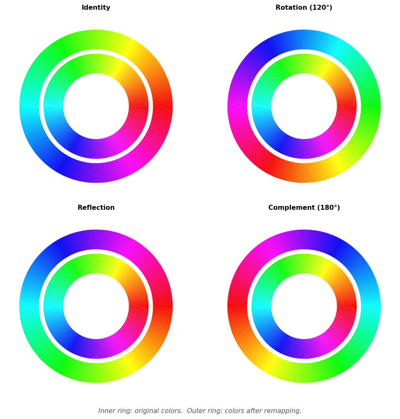
The color wheel has a few natural candidate automorphisms: rotations, reflections, and complement maps.

Figure 1: Color-wheel permutations: identity, rotation, reflection, and complement map.

If the color wheel were the whole story, then these automorphisms would work. Rotations and reflections are isometries of the circle. The inverted spectrum would be trivially possible, and pure functionalism would be in trouble.

But the color wheel is a cartoon model of human color perception. Does the empirical distance function on color space have any symmetries?

Chromaticity Diagrams

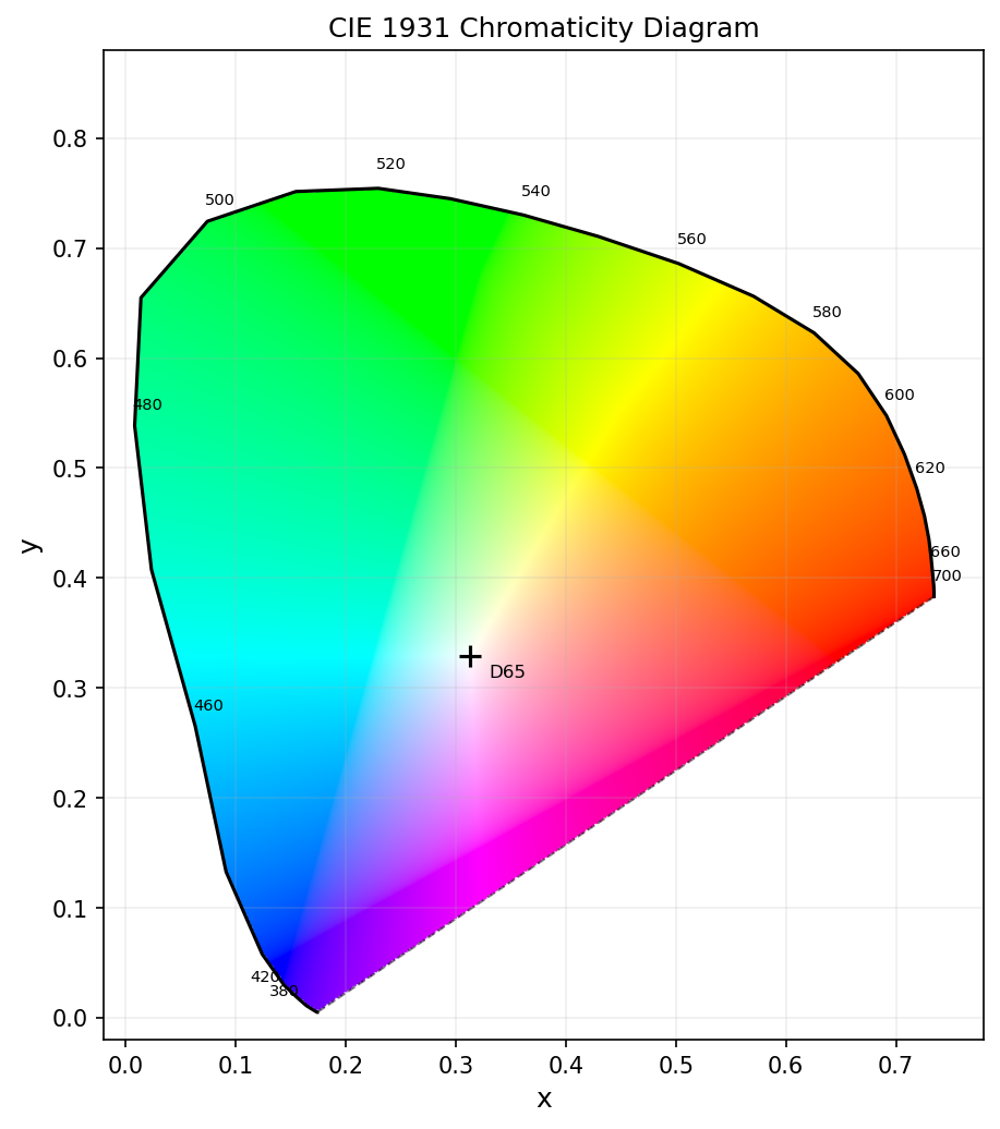
The CIE (Commission Internationale de l’Eclairage) chromaticity diagram, introduced in 1931, maps the visible colors onto a two-dimensional space². But the Euclidean distances in this diagram do not correspond to perceptual distances. Two colors that look wildly different might be close together in the diagram, and two that look similar might be far apart.

Figure 2: CIE 1931 Chromaticity Diagram. Euclidean distances in this space do not correspond to perceptual distances.

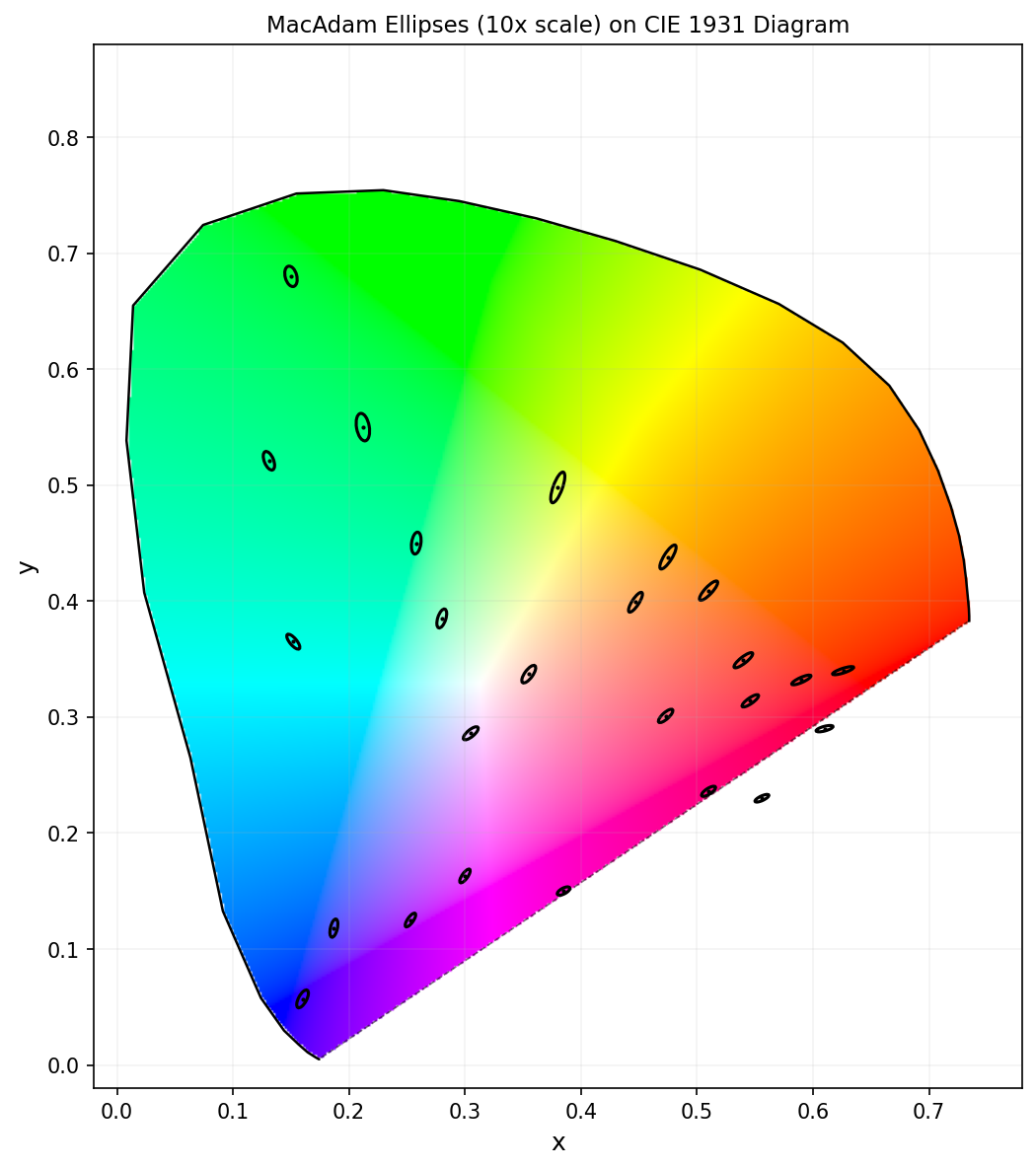
The mismatch between coordinate distance and perceptual distance means the metric changes from place to place. In 1942, David MacAdam measured this directly³. At various points in the CIE diagram, he tested subject’s ability to distinguish a color from a central color. Near green, the subjects were bad at discriminating, but near blue-violet, the subjects were very sensitive. The equivalent regions form ellipses of varying size, shape, and orientation across the diagram. These are the MacAdam ellipses.

Figure 3: MacAdam ellipses (shown at 10x actual size) on the CIE 1931 chromaticity diagram. The ellipses vary in size, shape, and orientation — the metric is non-uniform.

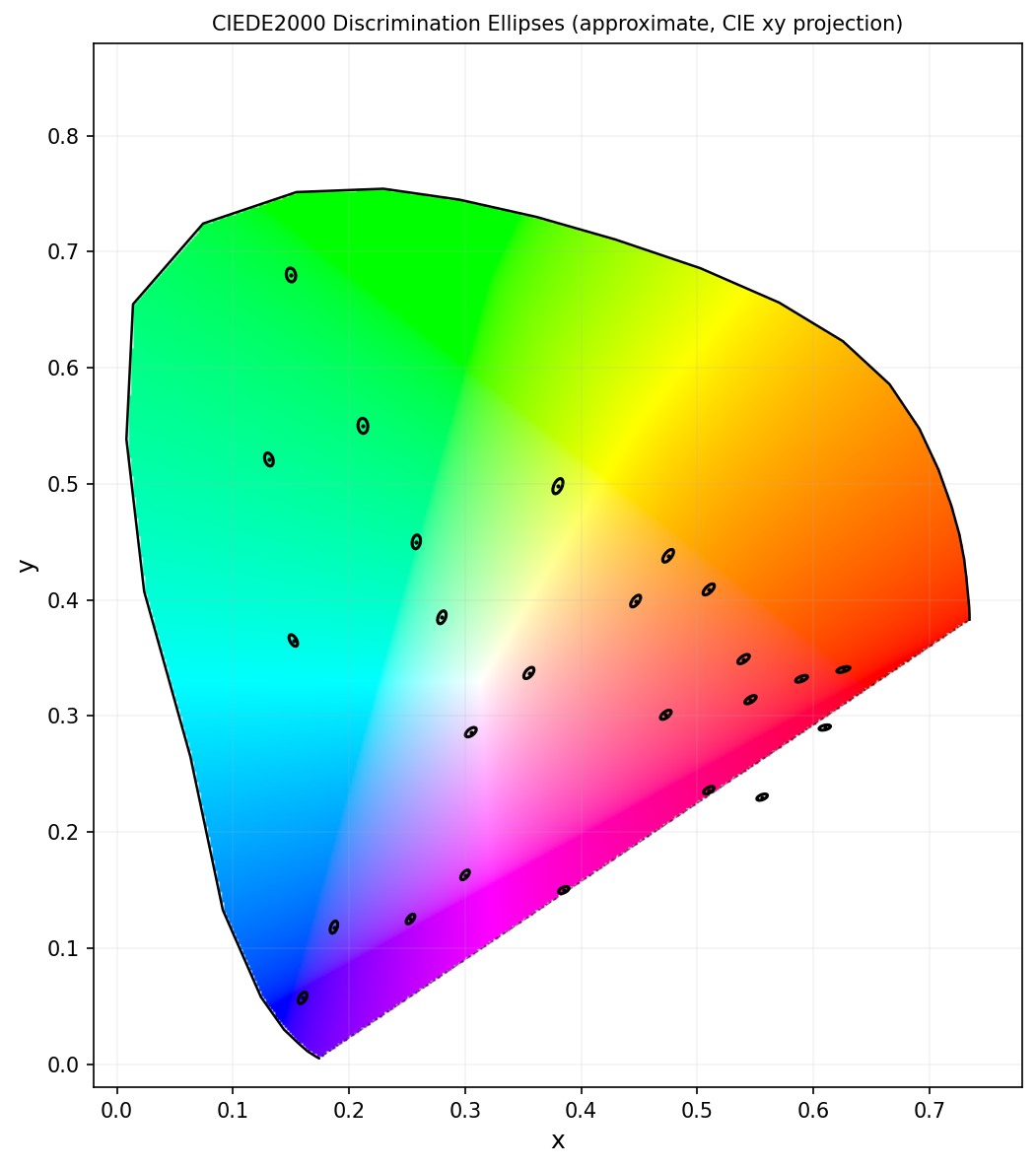
Subsequently, the CIE has released a series of increasingly sophisticated color difference formulas over the decades: CIELAB (1976), CIE94 (1994), and CIEDE2000 (2000)⁴. Each represents an improved approximation to the true perceptual metric, incorporating additional empirical data about how humans discriminate colors under various conditions. All of them confirm and refine MacAdam’s basic finding: the perceptual metric on color space is non-uniform and varies from region to region.

Figure 4: CIEDE2000 discrimination ellipses (approximate, projected onto CIE xy). More uniform than MacAdam’s original measurements, but still position-dependent. The metric has no global symmetry.

So we can think of color as a Riemannian manifold. The metric tensor encodes JND structure at each point, with large eigenvalues where discriminability is fine and small eigenvalues where discriminability is coarse. The MacAdam ellipses directly determine \(g_{ij}\) at each point, as the ellipse of just-noticeable differences is the unit ball of the local metric⁵.

A spectrum inversion that preserves all perceptual distances is an isometry \(\phi: M \to M\) with \(\phi^* g = g\). But it’s also true that⁶ for a generic Riemannian metric on a manifold of dimension \(\geq 2\), the only isometry is the identity.

Theorem. Let \(M\) be a smooth manifold of dimension \(n \geq 2\). The set of Riemannian metrics on \(M\) whose isometry group is trivial (i.e., \(\text{Isom}(M, g) = \{e\}\), consisting of only the identity) is generic: it is a residual set (countable intersection of open dense sets) in the space of all smooth metrics on \(M\), equipped with the \(C^\infty\) topology.

In plain language: if you pick a Riemannian metric “at random”⁷ from the space of all possible metrics, it will almost certainly have no non-trivial isometries. The only distance-preserving map from the space to itself will be the map that sends every point to itself.

In the Appendix, we provide computational evidence for this by fitting metric tensors from MacAdam’s ellipse data and searching for Killing vector fields (generators of continuous symmetries). No non-trivial solutions are found, consistent with a trivial continuous isometry group.

The Philosophical Payoff

What does this mean for the debate between functionalism and qualia realism?

The Riemannian argument shows that the inverted spectrum is not possible. The relational structure is rich enough to pin down the identity of each color up to the trivial isometry. There is no room for a non-trivial automorphism. If functional role includes the full discriminability structure, then two people who share the same color metric have the same color experiences. At least for color, the inverted spectrum is ruled out, and the case for functionalism over qualia realism is strengthened.

This is also evidence for structuralism. If the relational structure of color space has no non-trivial automorphisms, then there is no sense in which two colors could be “swapped” while preserving all the perceptual relations. In some sense, the “what it’s like” of red may be defined by its position in the web of perceptual relations⁸.

Individual Variation

The computation above addresses within-subject symmetry. Given one person’s color metric, can that person’s own color space be nontrivially remapped onto itself? But the assumption that “any two people [have] the same perceptual distance function” is doing a lot of work. The between-subject question is different. If two people have different JND structures (different metrics), can we still compare their color experiences?

Humans are not all alike. To start, trichromats, dichromats (i.e. color blind individuals), anomalous trichromats, and tetrachromats (people with four types of cone cells) all have different color spaces with different metrics. Secondly, the argument does not directly say that two different people must have the same color experiences. Two different people have two different manifolds with two different metrics. Comparing across individuals requires more than isometry theory: it requires some way to identify corresponding points across different metric spaces.

At a biological level, people have differing cone distributions, cone spectral sensitivities, lens and macular filtering, and different rod contributions in low-light regimes. Those differences imply slightly different empirical metrics. So the right conclusion is not “everyone sees exactly the same colors” but that (among people in the same phenotpyical category) colors differ by \(\epsilon\)-level distortion.

In short: we probably do see slightly different colors.

Conclusion

The inverted spectrum thought experiment asks: could two people have systematically different color experiences while being functionally identical? The traditional assumption is that this question is permanently open.

But color space is an empirical object with measurable geometry. The MacAdam ellipses show that this geometry is non-uniform and position-dependent, and a generic metric with these properties has no non-trivial isometries. If the color metric is generic (and the data strongly suggests it is) then there is no way to remap colors while preserving all perceptual distances.

We probably see close to, but not exactly, the same colors.

Caveats and Extensions

Is the Color Metric Actually Generic?

The theorem says a generic metric has no non-trivial isometries. But “generic” is a topological claim about the space of all metrics. The empirical question is whether the actual color metric, the one determined by MacAdam ellipses and CIE formulas, is in this generic set.

The empirical evidence is strongly suggestive. The MacAdam ellipses vary substantially and irregularly across the chromaticity diagram. There is no obvious axis of symmetry, no rotational invariance, no discrete symmetry group that jumps out of the data. But “strongly suggestive” is not a proof. In the Appendix, we search for Killing vector fields (generators of continuous symmetries) by fitting metric tensors from MacAdam’s ellipse data. No non-trivial solutions are found within a polynomial ansatz, which is suggestive but not conclusive, since the search is restricted to a finite-dimensional function class, and Killing fields only rule out continuous symmetries, not discrete ones.

Approximate Isometries

Perhaps the strongest objection: what if the inverted spectrum does not need to be exact? What if an approximate inversion is enough?

Define an \(\epsilon\)-isometry as a diffeomorphism \(\phi: M \to M\) such that:

\[ \sup_{x \in M} \| \phi^*g(x) - g(x) \| < \epsilon \]

For small \(\epsilon\), this is a map that almost preserves all perceptual distances. Could such a map exist even when exact isometries do not?

Possibly. If there exists a map that permutes colors while distorting each JND distance by a small amount, it might be the case that the distortion is below the threshold of detectability. This would give a “fuzzy” inverted spectrum. The inversion would be imperfect close enough to be undetectable in practice.

Whether such approximate isometries exist for the empirical color metric is an open question. It depends on how “close” the metric is to one with symmetry. One might study this via the space of Killing-like vector fields that satisfy \(\|\mathcal{L}_X g\| < \epsilon\) for small \(\epsilon\), an area sometimes called “approximate symmetry” in the physics literature.

If approximate isometries exist, the philosophical upshot is more subtle, and the debate would shift from “is inversion possible?” to “how much perceptual distortion is compatible with behavioral indistinguishability?”

Does JND Capture Everything?

The argument assumes that JNDs capture all perceptually relevant structure. But color experience might have structure that is not captured by pairwise discriminability. For example, there could be higher-order relations, temporal dynamics, or categorical boundaries that are not captured by JNDs alone.

For example, the “distance” between red and green might not fully capture the fact that they are “opponent” colors in a way that red and blue are not. Color opponency creates categorical structure that may not reduce to metric distances. However, opponent processing is itself a structural property. If red-green opponency is a feature of the wiring of the visual system, it provides additional constraints that make non-trivial remappings harder, not easier.

In general, if we enrich the structure of color space beyond the Riemannian metric, the automorphism group gets smaller, not larger. So these considerations, if anything, strengthen the conclusion.

Is Color Space Even Riemannian?

Recent work by Bujack et al. (2022) argues that perceptual color space is not Riemannian at all⁹. Large color differences are perceived as less than the sum of small differences, creating a “diminishing returns” effect that violates the path-additivity required by Riemannian geometry. If that’s correct, the MacAdam-ellipse metric is only valid locally (for small differences), and the global geometry requires a different framework.

If anything, this also strengthens the argument. The Riemannian case is the most symmetric possibility: a smooth, well-behaved metric with clean transformation properties. A non-Riemannian structure with diminishing returns is more irregular, making non-trivial distance-preserving self-maps even harder to construct. The Killing field computation above uses only local metric data and remains valid regardless.

Other Sensory Modalities

Does the argument generalize?

• Pitch: Pitch perception defines a metric space (JNDs for frequency discrimination). The octave structure introduces a periodicity, but the metric is non-uniform within an octave. Does pitch space have non-trivial isometries? The octave equivalence might generate a discrete isometry (translation by one octave), but this is not a “full inversion” and its existence is already part of the known structure.

• Taste and Smell: Taste and small are high-dimensional and poorly characterized metrically. The argument applies in principle, but we lack the empirical data to say whether the taste metric is generic.

• Pain: Pain has an intensity metric but unclear spatial or qualitative geometry. Same caveat.

The Quidditism Response

A committed quidditist can simply deny the premise. Qualia, they might say, have non-structural properties that no relational structure can capture. Even if the metric pins down the structural identity of each color, the intrinsic feel could still differ.

This is logically consistent. But it comes at a cost. If qualia have properties that make no difference to any relational, discriminative, or behavioral fact, then those properties are by definition epiphenomenal, and have no causal powers or no detectable consequences. The quidditist is committed to the existence of properties that are undetectable.

AI Disclosure

I used Claude to help research, draft, and edit this essay, based on my notes. Claude also devised several of the caveats and extensions, which I then edited and expanded on. Claude wrote the Killing field code in the appendix, which I then verified and modified. The related work survey was produced using ChatGPT Deep Research and then edited for accuracy.

Appendix A: Computing the Killing Fields

The theorem tells us that generic metrics have no symmetries. But is the empirical color metric generic? We can check directly by fitting a metric tensor from the MacAdam ellipse data and solving for Killing vector fields.

Each MacAdam ellipse defines the local metric tensor \(g_{ij}\) at its center: the ellipse of just-noticeable differences is the unit ball of the local metric. An ellipse with semi-axes \(a\), \(b\) and orientation \(\theta\) gives:

\[ g_{11} = \frac{\cos^2\theta}{a^2} + \frac{\sin^2\theta}{b^2} \] \[ g_{12} = \cos\theta\sin\theta\left(\frac{1}{a^2} - \frac{1}{b^2}\right) \] \[ \quad g_{22} = \frac{\sin^2\theta}{a^2} + \frac{\cos^2\theta}{b^2} \]

We interpolate between the 25 measurements to get a smooth metric field, then ask: does any smooth vector field \(X\) generate a flow that preserves all distances? Such a field must satisfy the Killing equation, so the Lie derivative of the metric along \(X\) vanishes:

\[ (\mathcal{L}_X g)_{ij} = X^k \partial_k g_{ij} + g_{kj} \partial_i X^k + g_{ik} \partial_j X^k = 0 \]

In 2D this gives 3 equations at every point:

\[ X^1 \partial_x g_{11} + X^2 \partial_y g_{11} + 2g_{11}\,\partial_x X^1 + 2g_{12}\,\partial_x X^2 = 0 \] \[ X^1 \partial_x g_{12} + X^2 \partial_y g_{12} + g_{12}\,\partial_x X^1 + g_{22}\,\partial_x X^2 + g_{11}\,\partial_y X^1 + g_{12}\,\partial_y X^2 = 0 \] \[ X^1 \partial_x g_{22} + X^2 \partial_y g_{22} + 2g_{12}\,\partial_y X^1 + 2g_{22}\,\partial_y X^2 = 0 \]

We parameterize \(X\) as a degree-3 polynomial vector field (20 unknown coefficients), evaluate the Killing equation at 332 grid points inside the gamut (\(3 \times 332 = 996\) constraints), and stack everything into an overdetermined linear system \(A\mathbf{c} = 0\). If a non-trivial Killing field existed within this polynomial ansatz, \(A\) would have a near-zero singular value. It doesn’t, though this is evidence against continuous symmetries within a restricted function class, not a proof of their absence.

import numpy as np
from scipy.interpolate import RBFInterpolator

# MacAdam (1942) ellipse data, Table III. 25 ellipses at 10-step magnification.
# Source: Wyszecki & Stiles (1982), Color Science, Table 5(5.4.1);
#         digitized via the LuxPy colour science library.
# Format: (x, y, semi-major a, semi-minor b, angle in degrees)
# Note: since the Killing equation is homogeneous (L_X g = 0), the 10x
# scaling factor cancels and does not affect whether solutions exist.
macadam_data = [
    (0.160, 0.057, 0.0085, 0.0035, 62.5),
    (0.187, 0.118, 0.0220, 0.0055, 77.0),
    (0.253, 0.125, 0.0250, 0.0050, 55.5),
    (0.150, 0.680, 0.0960, 0.0230, 105.0),
    (0.131, 0.521, 0.0470, 0.0200, 112.5),
    (0.212, 0.550, 0.0580, 0.0230, 100.0),
    (0.258, 0.450, 0.0500, 0.0200, 92.0),
    (0.152, 0.365, 0.0380, 0.0190, 110.0),
    (0.280, 0.385, 0.0400, 0.0150, 75.5),
    (0.380, 0.498, 0.0440, 0.0120, 70.0),
    (0.160, 0.200, 0.0210, 0.0095, 104.0),
    (0.228, 0.250, 0.0310, 0.0090, 72.0),
    (0.305, 0.323, 0.0230, 0.0090, 58.0),
    (0.385, 0.393, 0.0380, 0.0160, 65.5),
    (0.472, 0.399, 0.0320, 0.0140, 51.0),
    (0.527, 0.350, 0.0260, 0.0130, 20.0),
    (0.475, 0.300, 0.0290, 0.0110, 28.5),
    (0.510, 0.236, 0.0240, 0.0120, 29.5),
    (0.596, 0.283, 0.0260, 0.0130, 13.0),
    (0.344, 0.284, 0.0230, 0.0090, 60.0),
    (0.390, 0.237, 0.0250, 0.0100, 47.0),
    (0.441, 0.198, 0.0280, 0.0095, 34.5),
    (0.278, 0.223, 0.0240, 0.0055, 57.5),
    (0.300, 0.163, 0.0290, 0.0060, 54.0),
    (0.365, 0.153, 0.0360, 0.0095, 40.0),
]

# Convert each ellipse to metric tensor components
points, g11_vals, g12_vals, g22_vals = [], [], [], []
for (cx, cy, a, b, angle_deg) in macadam_data:
    theta = np.radians(angle_deg)
    c, s = np.cos(theta), np.sin(theta)
    g11 = (c/a)**2 + (s/b)**2
    g12 = c * s * (1/a**2 - 1/b**2)
    g22 = (s/a)**2 + (c/b)**2
    points.append([cx, cy])
    g11_vals.append(g11)
    g12_vals.append(g12)
    g22_vals.append(g22)

points = np.array(points)

# Interpolate each component using thin-plate splines
interp_g11 = RBFInterpolator(points, g11_vals, kernel='thin_plate_spline', smoothing=1.0)
interp_g12 = RBFInterpolator(points, g12_vals, kernel='thin_plate_spline', smoothing=1.0)
interp_g22 = RBFInterpolator(points, g22_vals, kernel='thin_plate_spline', smoothing=1.0)

def get_metric(x, y):
    pt = np.array([[x, y]])
    return np.array([[interp_g11(pt)[0], interp_g12(pt)[0]],
                     [interp_g12(pt)[0], interp_g22(pt)[0]]])

from matplotlib.path import Path

# CIE 1931 spectral locus (for determining which points are inside the gamut)
wl_x = np.array([0.1741,0.1740,0.1714,0.1644,0.1566,0.1440,0.1241,0.0913,0.0633,
    0.0235,0.0082,0.0139,0.0743,0.1547,0.2296,0.2950,0.3616,0.4294,0.5028,
    0.5706,0.6256,0.6658,0.6915,0.7079,0.7190,0.7260,0.7300,0.7320,0.7334,
    0.7344,0.7347,0.7347,0.7347])
wl_y = np.array([0.0050,0.0050,0.0065,0.0109,0.0177,0.0297,0.0578,0.1327,0.2650,
    0.4073,0.5384,0.6548,0.7243,0.7514,0.7543,0.7449,0.7300,0.7106,0.6858,
    0.6562,0.6229,0.5858,0.5475,0.5123,0.4813,0.4562,0.4353,0.4188,0.4044,
    0.3935,0.3872,0.3848,0.3830])
locus_path = Path(np.column_stack([np.append(wl_x, wl_x[0]), np.append(wl_y, wl_y[0])]))

# Build grid inside the gamut
grid_pts = []
for xi in np.linspace(0.10, 0.65, 20):
    for yi in np.linspace(0.08, 0.65, 20):
        if locus_path.contains_point((xi, yi)):
            grid_pts.append((xi, yi))
grid_pts = np.array(grid_pts)

def poly_basis(x, y, degree=3):
    """Monomials up to given degree: 1, x, y, x^2, xy, y^2, ..."""
    basis = []
    for i in range(degree + 1):
        for j in range(degree + 1 - i):
            basis.append(x**i * y**j)
    return np.array(basis)

h = 0.005  # finite difference step
deg = 3
n_basis = len(poly_basis(0, 0, deg))  # = 10
n_params = 2 * n_basis                 # = 20

# Assemble the constraint matrix: 3 Killing equations per grid point
rows = []
for (px, py) in grid_pts:
    g = get_metric(px, py)
    dg_dx = (get_metric(px+h, py) - get_metric(px-h, py)) / (2*h)
    dg_dy = (get_metric(px, py+h) - get_metric(px, py-h)) / (2*h)

    phi = poly_basis(px, py, deg)
    dphi_dx = (poly_basis(px+h, py, deg) - poly_basis(px-h, py, deg)) / (2*h)
    dphi_dy = (poly_basis(px, py+h, deg) - poly_basis(px, py-h, deg)) / (2*h)

    # (L_X g)_ij = X^k dk(g_ij) + g_kj di(X^k) + g_ik dj(X^k)
    for i, j in [(0,0), (0,1), (1,1)]:
        row = np.zeros(n_params)
        # Term 1: X^k partial_k g_ij
        row[:n_basis] += phi * dg_dx[i,j]   # X^1 contribution
        row[n_basis:] += phi * dg_dy[i,j]   # X^2 contribution
        # Term 2: g_kj partial_i X^k
        di = [dphi_dx, dphi_dy][i]
        row[:n_basis] += g[0,j] * di
        row[n_basis:] += g[1,j] * di
        # Term 3: g_ik partial_j X^k
        dj = [dphi_dx, dphi_dy][j]
        row[:n_basis] += g[i,0] * dj
        row[n_basis:] += g[i,1] * dj
        rows.append(row)

A = np.array(rows)

# Solve via SVD: any Killing field lives in the null space of A
U, S, Vt = np.linalg.svd(A, full_matrices=True)

Results

If a non-trivial Killing field existed, the matrix \(A\) would have a near-zero singular value, a direction in parameter space that (approximately) satisfies all 996 constraints. Here are the singular values:

Index	Singular value	Ratio to \(\sigma_{\max}\)
0	\(1.85 \times 10^6\)	1.0000
1	\(8.47 \times 10^5\)	0.4578
2	\(5.11 \times 10^5\)	0.2764
3	\(3.70 \times 10^5\)	0.2002
4	\(2.66 \times 10^5\)	0.1440
5	\(1.96 \times 10^5\)	0.1057
6	\(1.31 \times 10^5\)	0.0708
7	\(1.10 \times 10^5\)	0.0595
8	\(9.34 \times 10^4\)	0.0505
9	\(5.48 \times 10^4\)	0.0296
10	\(3.04 \times 10^4\)	0.0164
11	\(2.42 \times 10^4\)	0.0131
12	\(1.76 \times 10^4\)	0.0095
13	\(1.72 \times 10^4\)	0.0093
14	\(1.25 \times 10^4\)	0.0068
15	\(1.03 \times 10^4\)	0.0055
16	\(5.61 \times 10^3\)	0.0030
17	\(4.19 \times 10^3\)	0.0023
18	\(2.32 \times 10^3\)	0.0013
19	\(1.75 \times 10^3\)	0.0009

The smallest singular value is \(\sigma_{19} = 1.75 \times 10^3\), with a ratio of \(9.5 \times 10^{-4}\) relative to the largest. The singular values decay smoothly with no sharp drop toward zero, which is what we would expect if no non-trivial Killing field exists within the polynomial ansatz.

Caveats: the absolute magnitudes of the singular values depend on coordinate scaling, ellipse conventions, and interpolation choices, so “three orders of magnitude” should not be over-interpreted. Killing fields detect only continuous symmetries; a discrete isometry (e.g., a reflection) would not appear as a Killing field. And the degree-3 polynomial parameterization, while generous (a Killing field on a 2-manifold is determined by 3 parameters), is still a restricted function class. The computation is best read as evidence consistent with the generic-metric theorem, not as an independent proof.

Appendix B: Related Work and Novelty

Related Work

The inverted spectrum is one of the most extensively discussed thought experiments in philosophy of mind. The Stanford Encyclopedia of Philosophy entry on inverted qualia surveys the landscape of structural and empirical constraints on inversion scenarios¹⁰. Philosophers have long noted that real color perception is not a simple hue circle but a structured, asymmetric quality space, and that these asymmetries undermine naive “hue rotation” models of inversion.

On the empirical side, perceptual color differences have been studied since MacAdam’s 1942 measurements of discrimination ellipses in CIE space¹¹. These ellipses are widely interpreted as defining a local perceptual metric. Modern color difference formulas such as CIEDE2000 formalize this further¹².

Several authors treat color discrimination geometry in explicitly differential-geometric terms. Gravesen (2015) models MacAdam ellipses as defining a Riemannian metric and studies coordinate constructions that approximate perceptual uniformity¹³. Chevallier and Farup (2018) analyze how MacAdam ellipses should be interpolated to produce a consistent metric tensor field, showing that naive interpolation can be geometrically misleading¹⁴. Bujack et al. (2022) argue that perceptual color space may not be globally Riemannian at all, due to violations of path additivity for large color differences¹⁵.

In differential geometry, the generic triviality of isometry groups for smooth Riemannian manifolds is a classical result¹⁶. Non-trivial self-symmetries of generic metrics are exceptional rather than typical.

Novelty

The philosophical literature contains informal asymmetry arguments against simple inverted spectrum models. The color science literature contains metric and geometric analyses of perceptual color space. I arrived at the argument in this essay independently before discovering the geometric color science literature, and to my knowledge the two threads have not been combined in the way proposed here.

What is distinctive here is threefold:

1. Formalization: Undetectable inversion is identified with a non-trivial isometry of empirical perceptual geometry. Rather than arguing from qualitative asymmetry, the condition is made mathematically precise.

2. Reduction to symmetry detection: If inversion requires a non-trivial automorphism, then the question becomes whether the empirically fitted perceptual metric admits such symmetries. The generic-metric theorem answers this in the negative for “almost all” metrics.

3. A computational test: The Killing field computation in the preceding appendix treats inversion as a concrete question about the symmetry group of a metric estimated from discrimination data.

The underlying empirical and geometric components are established in prior work. The novelty lies in reframing the inverted spectrum debate as a problem about the symmetry structure of perceptual geometry and proposing concrete methods to evaluate it.

Footnotes

1. This is similar to the axiom of function extensionality in type theory, which says that two functions are equal if they give the same outputs for all inputs. The functionalist is committed to a kind of extensionality for mental states: if all inputs and outputs are the same, the states are the same.

2. The full color space is three-dimensional (hue, saturation, brightness), but much of the key structure can be seen in the two-dimensions, holding brightness constant.

3. MacAdam, D. L. (1942). “Visual Sensitivities to Color Differences in Daylight.” Journal of the Optical Society of America, 32(5), 247–274.

4. Sharma, G., Wu, W., and Dalal, E. N. (2005). “The CIEDE2000 color-difference formula: Implementation notes, supplementary test data, and mathematical observations.” Color Research & Application, 30(1), 21–30.

5. Treating MacAdam ellipses as defining a Riemannian metric is standard in color science. See Gravesen, J. (2015), “The metric of colour space,” Graphical Models, 82, 77-86. Chevallier, E. and Farup, I. (2018), “Interpolation of the MacAdam Ellipses,” SIAM Journal on Imaging Sciences, 11(3), 1979-2000, show that naive component-wise interpolation of the metric tensor can be geometrically misleading; proper interpolation requires care about the manifold structure of the space of positive-definite matrices.

6. See, e.g., Kobayashi, S. (1972). Transformation Groups in Differential Geometry. Springer-Verlag. Also: Ebin, D. G. (1970). “The manifold of Riemannian metrics.” Proceedings of Symposia in Pure Mathematics, Vol. 15, AMS.

7. “Generic” here is used in the topological sense, not the probabilistic sense. But the intuition is similar: non-trivial isometries require the metric to satisfy special symmetry conditions, and these conditions are rare. Color space is effectively compact (bounded by the spectral locus), so the standard genericity results apply. Metrics that do have non-trivial isometries, like the sphere, Euclidean space, or hyperbolic space, are very special, and they have enormous amounts of symmetry. A generic metric, without special structure, has no symmetry at all.

8. This connects to broader structuralist positions in philosophy of science and metaphysics. See, e.g., Ladyman, J. (2014). “Structural Realism.” Stanford Encyclopedia of Philosophy. The idea that physical (or experiential) properties are individuated by their structural roles has a long history.

9. Bujack, R., Teti, E., Miller, J., Caffrey, E., and Turton, T. L. (2022). “The non-Riemannian nature of perceptual color space.” Proceedings of the National Academy of Sciences, 119(18), e2119753119.

10. Tye, M. (2025). “Inverted Qualia.” Stanford Encyclopedia of Philosophy.

11. MacAdam, D. L. (1942). “Visual Sensitivities to Color Differences in Daylight.” Journal of the Optical Society of America, 32(5), 247–274.

12. Sharma, G., Wu, W., and Dalal, E. N. (2005). “The CIEDE2000 color-difference formula: Implementation notes, supplementary test data, and mathematical observations.” Color Research & Application, 30(1), 21–30.

13. Gravesen, J. (2015). “The metric of colour space.” Graphical Models, 82, 77-86.

14. Chevallier, E. and Farup, I. (2018). “Interpolation of the MacAdam Ellipses.” SIAM Journal on Imaging Sciences, 11(3), 1979-2000.

15. Bujack, R., Teti, E., Miller, J., Caffrey, E., and Turton, T. L. (2022). “The non-Riemannian nature of perceptual color space.” Proceedings of the National Academy of Sciences, 119(18), e2119753119.

16. See, e.g., Kobayashi, S. (1972). Transformation Groups in Differential Geometry. Springer-Verlag. Also: Ebin, D. G. (1970). “The manifold of Riemannian metrics.” Proceedings of Symposia in Pure Mathematics, Vol. 15, AMS.