This page will continue to be updated over the next week as results from subsequent experiments come in.

Anicet Charles Gabriel Lemonnier, *In the Salon of Madame Geoffrin in 1755* (1812).

Introduction

As machine-learning systems saturate benchmarks and make generation abundant, the bottleneck in many domains has shifted from “doing work” to “evaluating whether the work done is good.”¹

¹ For related essayistic discussions of specification, taste work, and the social formation of evaluative standards, see my other writings such as The Paradox of Taste, How Will Humans Generate Value In a Post-AI Society?, and Functional Explanations of Art.

² Amusingly, in the Baihais experiment, the first set of critical standards the agents settled on involved “counting”: quantitatively checking to see if a generated image has the exact number of an object mentioned in the caption. They then proceeded to develop more advanced methods of checking an image against the caption. This is a miniature version of the same problem: while formalizable criteria are easy to coordinate around, they don’t necessarily produce satisfying outputs. This may also result in problems in human society.

In some domains, such as software and math, there are machine-checkable methods for identifying whether or not a machine-generated output is correct according to formal criteria. But correctness (“does this object match its specification?”) is in some sense the least possible form of evaluation². There are an infinitude of true theorems and valid programs, the vast majority of which are ugly, uninteresting, and/or useless. A verifier can tell us whether an output is admissible, but can’t tell us whether the output was worth producing in the first place.

This doesn’t mean that evaluations lacking formal verification are arbitrary. While opinions can’t be right or wrong, they can be good or bad. Judgments can be informed or naive, perceptive or superficial, fruitful or sterile, novel or cliche. Even without a formal verifier, judgments may contain useful structure.

This is especially relevant in fuzzy, qualitative domains like art, where qualities like elegance or beauty lack formal definitions or carry a contextual element. And fuzziness is not the only source of difficulty. We also lack formal evaluation criteria in domains where the relevant consequences arrive only after a long delay or long-horizon, open-ended questions (for example, “is it good to study chemical engineering?” or “what makes a good life?”). Frontier science and mathematics face a similar problem: a result may be correct without being important, and recognizing its significance may require concepts or expertise that human evaluators have yet to develop.

The usual response to these limitations is to put a human in the loop, often using techniques such as RLHF or labeled data. But this only pushes the problem back one step. Where did the human evaluator’s standards come from in the first place? If AI systems are to exercise judgment in new and unfamiliar domains, they may need a comparable capacity to develop evaluative standards rather than merely inherit them³. Relatedly, we want to ensure that AI judgments of “good” and “bad”, and their processes for developing new such judgments, are aligned with humans’, especially for moral questions.

³ “Evaluator” here is some function that maps on objects, outcomes, or trajectories into “judgments”. This might be a scalar reward function but we can’t rule out contextual, pairwise, incomplete, plural, or cyclic evaluators (more on this in future work, but there’s lots of work in the literature on this).

Social Learning

There is nothing either good or bad, but thinking makes it so.

— William Shakespeare, Hamlet, Act II, Scene 2

The problem of learning good judgment ex nihilo is deeper and harder than mimicking a given human reward function. One issue is that human evaluators aren’t fixed: they change through exposure. As people learn what possibilities exist, which distinctions matter, and what deserves attention, they may adjust their goals and values. Thus, evaluation is entwined with representation: agents must learn the objects and distinctions over which preferences can be expressed before they can express preferences over them, and they may change their preferences by changing the vocabulary through which they view the world.

Common reinforcement learning concepts such as regret become harder to define if the reward function itself is malleable. Standard RL usually models this as maximizing expected return. We use metrics like “regret” to evaluate how much worse an agent’s choices were than the best available policy under a fixed reward function:

\[ \operatorname{Regret}(K) =\sum_{k=1}^{K}\left[V^*(s_0)-V^{\pi_k}(s_0)\right] \]

Here \(V^\pi(s_0)\) is expected episode return, \(V^*(s_0)\) is the optimal expected return, and \(\pi_k\) is the policy used in episode \(k\). All \(K\) episodes start at \(s_0\).

But if experience changes the evaluator, the standard against which those choices are judged also changes. An optimal action under an agent’s earlier values may be condemned by the agent’s later values. For a fixed recorded trajectory \(\tau\), the change in return is:

\[ G_{r'}(\tau)-G_r(\tau) =\sum_{t=0}^{T-1}\gamma^t \left[r'(s_t,a_t,s_{t+1})-r(s_t,a_t,s_{t+1})\right] \]

Here \(G_r(\tau)\) is the discounted return of the same recorded history under reward function \(r\). Changing \(r\) to \(r'\) can change their evaluation, but the difference can also be zero.

In ordinary regret analysis, the consequences of unchosen actions stay counterfactual. Humans experience only one trajectory and must estimate what would have happened along the others. Artificial agents need not share this limitation, since (given a simulator) an agent can be copied before a decision and each copy can be sent down a different path. In principle, this makes it possible to observe rather than just imagine the consequences of every available choice.

But what happens if each trajectory changes not only what the copy knows, but what it values? The branches can return with different evaluators, each applying a different standard to the original decision. Copying can reveal every possible outcome without revealing which outcome the original agent should prefer.

But regret is more than one evaluator disagreeing with another. To regret a choice, the agent evaluating it later must in some sense be the “same agent” as the agent that made the choice. Otherwise, the later evaluator is not regretting the earlier decision, but rather applying different preferences to someone else’s choice. If we want to compare judgments across copies, we have to assume that there is some factor that remains invariant as the agent changes.

This invariant can’t be the agent’s entire set of preferences, since then agents could never learn. But enough must remain stable for the agent’s changing judgments to count as revisions by one evaluator rather than the replacement of one evaluator by another. Let us consider this invariant quantity to be the “identity” of the agent⁴. Without identity, copying gives us many informed judgments, but no single agent capable of learning from all of them.

⁴ This is a provisional connection to a broader research program. Possibly these sorts of techniques apply both to individual identity and institutional identity. More speculatively, identity might be compared to a conserved quantity associated with invariance through time (ideally some Noetherlike derivation would work here but it’s out of scope of this post).

The identity constraint means that judgments from divergent copies can’t just be pooled as though they came from one evaluator. Whether the copies remain versions of the same agent depends on what (if anything) remains invariant across their different trajectories. When they do become distinct evaluators, however, their experiences may still be useful to one another.

A full population explores more trajectories than an individual agent can realize. A learner can use other agents’ choices to estimate what would have happened had the learner acted differently. After changing their values, the learner can also reassess their own past experiences. Using a peer’s experience requires deciding whether the peer’s circumstances are comparable to the learner’s and which differences matter.

In order to get agents to learn like this, we need a different learning loop from the one usually considered in reinforcement learning. On the one hand, policy learning asks how an agent should act given an evaluator. On the other hand, evaluator learning asks how experience should change what the agent notices, compares, and values. The two processes are coupled: the evaluator determines which actions the agent takes and which experiences it encounters, while those experiences may in turn revise the evaluator.

In a population, those experiences include other agents and their judgments. This loop contains no supplied reward, yet one part of it is never revised: the environment, which fixes what follows from each action and which agents are present to be observed. What a population comes to value therefore depends on the environment and the rules of interaction, although neither specifies a reward.

The question is then how a learner can revise their evaluator using other agents’ judgments without simply adopting another agent’s evaluator. So we can try to cast evaluator formation as a problem of Social Learning⁵ ⁶.

⁵ Social interaction doesn’t automatically supply the right evaluator. A social game can stabilize conformity or error as easily as good judgment. How can we make the information and incentives of the social game track the relevant ontological structure without installing that structure as a hidden reward?

⁶ The phrase social learning has several established meanings. The use here focuses specifically on a machine learning paradigm by which multiple agents coevolve their evaluators. It bears some resemblance to concepts from economics and cultural evolution, where agents infer from observing and exchanging information with other agents.

Machine Social Learning

Humans develop and revise their judgments through social processes like imitation, comparison, and criticism.⁷ Given an agent equipped with an evaluation procedure, these processes expose the agent to judgments formed along other trajectories. The agent can accept or reject those judgments, or revise its own standards in response. Some of these judgments may be organized and sustained across people and time by institutions, which preserve accumulated judgments and establish practices through which standards are taught⁸.

⁷ Beyond transmitting standards, these processes might even create values that would not otherwise exist. Consider a one-shot trade. If two parties only ever engage once, the buyer needs a verifiable proxy for the utility that the product will deliver. If no adequate proxy exists (i.e. slow or tacit goods), then the buyer is forced to fall back to an existing proxy. Repeated relationships can avoid this by building trust: if you’ve eaten at a restaurant, you trust the chef to make a good meal. If your friend who you know has good taste recommends a restaurant, you can be assured that the restaurant is good. For goods whose utility must be learned (or even those beyond your capacity to learn, like an advanced math problem in a different field), this matters even more: you cannot judge the good until you have invested the attention to learn it, and a trusted recommendation is what makes that investment worth making before the payoff is visible. Thus, we can reason that dense, trusted networks are better at sustaining goods whose utility has to be learned.

⁸ For instance, scientific fields, firms, and artistic traditions may provide useful comparison cases. Members can turn over while recognizable standards of evidence, quality, or judgment persist.

⁹ Christiano et al. (2017), Deep Reinforcement Learning from Human Preferences, learn a reward model from human comparisons between trajectory segments and use that model to train a policy.

¹⁰ Related work lets agents learn to reward one another: Yang et al. (2020), Learning to Incentivize Other Learning Agents. Their incentive functions are trained to improve each reward-giving agent’s supplied external objective through changes in the other agents’ learning.

Machine learning systems already learn models of value. In preference-based reinforcement learning and RLHF, human comparisons are used to estimate a reward function that can guide policy optimization.⁹ Those comparisons are ordinarily treated as external evaluative evidence. Here, the learning problem includes the process that produces and changes the evaluators from which that evidence is collected. The central question is whether interaction can produce new evaluative structure, rather than merely elicit structure already latent in some external data.¹⁰

Imagine an attempt to build AlphaTaste, an artificial agent capable of developing new, coherent, distinctive, and transferable evaluative standards using only a seed corpus of materials. More speculatively, AlphaTasteZero would be a population of agents that bootstraps evaluative structure purely through social interaction and self-play from a thin or vacuous initial seed, without an externally supplied task reward¹¹. How would such a system operate, and how would we recognize good or even superhuman judgment if it developed?

¹¹ Here, “Zero” would mean proceeding without an externally supplied task reward that settles the evaluative question in advance. Presumably we still need some structure (things like the architecture, priors, memory, other agents, environmental dynamics, and rules governing what persists). The question is how thin and domain-general we can make these inputs.

This also suggests a possible mode of attack on the AI alignment problem. Instead of putting a fixed human value function directly into models, we can align the processes through which humans and AI systems develop and revise values. Aesthetics offers a comparatively safe testbed for this possibility. This avoids the problem of treating one person’s judgments (or proxies thereof) as the ultimate standards by which behavior is judged.

This post investigates preliminary mathematical and software frameworks for solving this problem. The aims are to construct new aesthetics and, ideally, to obtain recognizable points of coordination through the learning dynamics. Agreement alone and novelty alone would not establish both.

Mathematical Preliminaries

In order to distinguish prediction from evaluation, we will start with one agent making one decision. We will then go on to describe how the agent’s predictive and evaluative capabilities change over time.

Single Agent

Consider a single agent interacting with a fully observed environment with finite state space \(\mathcal S\), finite action space \(\mathcal A\), and environment transition kernel \(P\). The learner’s internal state at time \(t\) is described by \(z_t\):

\[ z_t=(\widehat P_t,r_t,\pi_t,C,m_t) \]

\(\widehat P_t\) is the learner’s predictive model. In a fully observed setting, \(\widehat P_t(s'\mid s,a)\) estimates the probability of successor state \(s'\) after action \(a\) in state \(s\).
\(r_t\) is the learner’s evaluative state, the reward model \(r_t(s,a,s')\) used to assess a transition.
\(\pi_t\) is the learner’s current policy. \(\pi_t(a\mid s)\) gives the probability of selecting action \(a\) in state \(s\).
\(C\) is the learning procedure that determines how experience updates the learner’s internal state.¹²
\(m_t\) is any retained memory or logs of past events (agents may choose to retain memories).

¹² The learning procedure \(C\) is held fixed here. In principle, we could also have agents learn their update procedure (socially).

These components describe functional roles within a learner and may share parameters or representations. A policy may choose actions by predicting and evaluating their consequences, or it may learn directly from trials without using a predictive model. In the latter case, the predictive-model component can be left unused. Both are choices within the same specification.

At each time step \(t\), the learner uses the policy contained in \(z_t\) to act in environment state \(S_t\), then updates their internal state from the resulting experience:

\[ \begin{aligned} A_t&\sim\pi_t(\cdot\mid S_t)\\ S_{t+1}&\sim P(\cdot\mid S_t,A_t)\\ e_t&=(S_t,A_t,S_{t+1})\\ d_t&=(e_t,B_t)\\ z_{t+1}&\sim K_C(\cdot\mid z_t,d_t) \end{aligned} \]

Here \(e_t\) records the interaction, \(B_t\) is optional incoming data, and \(K_C\) is the update kernel specified by \(C\).

The policy \(\pi_t\) is part of the learner’s internal state \(z_t\). After the update, the learner has internal state \(z_{t+1}\) and policy \(\pi_{t+1}\).

Incoming data may be empty, or a batch may contain unlabeled examples or labeled examples or other information¹³.

¹³ Labeled examples seem like they defeat the purpose; these are included here only to make it more obvious that this framework generalizes existing ML frameworks.

In fact, the external dataset is completely optional, and updates need not follow an action by the learner. When the learner receives data without acting in the environment, \(e_t\) is empty and the update uses the incoming batch \(B_t\). The transition and action-selection steps are then unnecessary.

The environment specifies the consequences of a given action. Each agent evaluates outcomes using their current reward model \(r:\mathcal S\times\mathcal A\times\mathcal S\to\mathbb R\).

Now, let us consider an episode with a single decision. Under a bounded reward model \(r\), the action value is

\[ Q_r^{(1)}(s,a) =\sum_{s'}P(s'\mid s,a)r(s,a,s') \]

An agent learning about the environment approximates the environment transition kernel \(P\) with an estimate \(\widehat P\), giving the estimated action value

\[ \widehat Q_r^{(1)}(s,a) =\sum_{s'}\widehat P(s'\mid s,a)\,r(s,a,s') \]

There are two ways the model can be updated:

Agent updates \(\widehat P\) to revise their predictions
Agent updates \(r\) to revise their evaluations.

Note that both \(\widehat P\) and \(r\) may be parametrized.

Agents choose actions using the policy \(\pi(a\mid s)\), which governs the actions they take.

As an example, suppose there are two possible terminal states, \(s_1\) and \(s_0\), and the evaluator assesses only the terminal state. Let \(\widehat p_a=\widehat P(s_1\mid s,a)\). Comparing actions \(a\) and \(b\), we obtain

\[ \begin{aligned} \widehat Q_r^{(1)}(s,a)-\widehat Q_r^{(1)}(s,b) &=\widehat p_a r(s_1)+(1-\widehat p_a)r(s_0)\\ &\quad-\widehat p_b r(s_1)-(1-\widehat p_b)r(s_0)\\ &=(\widehat p_a-\widehat p_b) \bigl[r(s_1)-r(s_0)\bigr] \end{aligned} \]

The first factor expresses the agent’s belief about which action is more likely to produce \(s_1\). The second expresses their preference for \(s_1\) over \(s_0\). Either factor can change sign and reverse the ranking of the actions. So an agent can change their preferred action while retaining the same evaluations or while retaining the same predictions.

Multiple Agents

Let us now extend the situation to \(n\) agents.

Index each learner’s state and update by \(i\in\{1,\ldots,n\}\). So:

\[ z_{i,t}=(\widehat P_{i,t},r_{i,t},\pi_{i,t},C_i,m_{i,t}) \] and \[ z_{i,t+1}\sim K_{C_i}(\cdot\mid z_{i,t},d_{i,t}) \]

In the multi-agent case, agents may use different learning procedures and may receive different records. The joint action of all agents is denoted \(\mathbf A_t=(A_{1,t},\ldots,A_{n,t})\).

Agents share an environment, which responds to the joint action through

\[ S_{t+1}\sim P(\cdot\mid S_t,\mathbf A_t) \]

Agents are coupled due to the shared transition and the experience made available to each learner.

We must also describe how the agents are coupled. Collect the environment and learner states:

\[ Z_t=(S_t,\mathbf O_t,\mathbf z_t) \]

Here \(O_{i,t}\) is the information available to agent \(i\). Under full observation \(O_{i,t}\) includes \(S_t\), but otherwise we need some additional restriction rule based on observation and retained memory.

Finally, let \(\mathsf E(s',\mathbf o',\mathbf B\mid Z,\mathbf a)\) denote the joint transition kernel for the next environment state, observations, and incoming data batches. In an interactive round the state marginal agrees with the environmental transition \(P(s'\mid s,\mathbf a)\). Source selection and correlations between agents’ data are included in \(\mathsf E\).

Specification

We’ve now reviewed a fair amount of notation, but not the type signatures on each element or how to specify them. To formulate a social learning problem, what specific elements must we specify?

Let \(\Delta(X)\) denote probability distributions on \(X\), \(\delta_x\) a point mass at \(x\), and \(X^*\) finite sequences of elements of \(X\), including the empty sequence \([]\). Each function below has a specified domain and codomain.

Spaces and Records

Choose a population size \(n\geq1\). For the fully observed setting, each agent observes the environment state \(S_t\). However, partial information is also possible.

Element	Type or definition	Example
Environment state \(S_t\)	\(S_t\in\mathcal S\); specify the state space (finite in this example)	\(\mathcal S=\{0,1\}\)
Agent action \(A_{i,t}\)	\(A_{i,t}\in\mathcal A_i\); choose a finite set \(\mathcal A_i\)	\(\mathcal A_i=\{0,1\}\)
Joint action \(\mathbf A_t\)	\(\mathbf A_t\in\mathcal A:=\prod_{i=1}^n\mathcal A_i\)	For two agents, \((A_{1,t},A_{2,t})=(0,1)\)
Evaluator class \(\mathcal R_i\)	\(\mathcal R_i\subseteq\{r:\mathcal S\times\mathcal A_i\times\mathcal S\to\mathbb R\}\); choose the admissible reward models	\(\mathcal R_i=\{(s,a_i,s')\mapsto\lambda(2s'-1):\lambda\in[-1,1]\}\) for the scalar evaluator illustrated below
Incoming batch \(B_{i,t}\)	\(B_{i,t}\in\mathcal B_i\); choose the batch type, including an empty batch. Each datum comes from external data or from another learner	With datum space \(\mathcal X_i=\mathcal S\), take \(\mathcal B_i=\mathcal X_i^*\); \(B_{i,t}=[0,1,1]\) or \([]\)
Interaction record \(e_{i,t}\)	\(e_{i,t}\in\mathcal E_i:=(\mathcal S\times\mathcal A_i\times\mathcal S)\sqcup\{\varnothing\}\)	\((0,1,1)\) for an observed transition; \(\varnothing\) for no interaction
Experience \(d_{i,t}\)	\(d_{i,t}\in\mathcal D_i:=\mathcal E_i\times\mathcal B_i\)	\(d_{i,t}=((0,1,1),[])\) or \((\varnothing,[0,1,1])\)
Memory \(m_{i,t}\)	\(m_{i,t}\in\mathcal M_i\); choose the retained representation	\(\mathcal M_i=\mathcal D_i^*\) retains a history; \(\mathcal M_i=\{\varnothing\}\) retains no separate memory

The finite spaces keep the example simple. Continuous physical states, such as CartPole’s position and angle, use measurable spaces and transition kernels, with integrals replacing the corresponding sums.

The table gives an evaluator for one transition. To score a whole performance, specify a record space \(\mathcal T_i\) and a scoring rule \(G_{r_i}:\mathcal T_i\to\mathbb R\) determined by the evaluator. For example, with discount factor \(0\leq\gamma\leq1\), a finite record \(\tau=(x_1,\ldots,x_T)\) can be assessed by

\[ G_{r_i}(\tau)=\sum_{k=1}^{T}\gamma^{k-1}r_i(x_k) \] \[ x_k=(s_{k-1},a_{i,k-1},s_k). \]

A score based on the pattern of motion over an entire performance need not have this additive form. Its features and scoring rule must be defined, and its records must retain the required history. The evaluator class must then be specified for those records. The Bellman derivation below concerns the additive case.

For a source \(j\), a reported comparison contains two records and a preference label obtained by comparing their scores under \(G_{r_j}\). The label is data in \(B_{i,t}\), distinct from the receiving learner’s evaluator \(r_{i,t}\) and from either numerical score.

No averaging rule is required by the learning loop. If an experiment uses one, we must specify what is averaged and over which observations. We must also distinguish these learned assessments from diagnostics used to describe the results: a test for balancing need not appear in the agent’s evaluator.

Learner Components

Let \(\mathcal Z_i\) denote the admissible tuples \(z_i=(\widehat P_i,r_i,\pi_i,C_i,m_i)\) with the component types below. The learning procedure \(C_i\) specifies the learner update kernel \(K_{C_i}\), held fixed during a training run.

Element	Type signature	Example
Predictive model \(\widehat P_{i,t}\)	\(\widehat P_{i,t}:\mathcal S\times\mathcal A_i\to\Delta(\mathcal S)\) when used; otherwise an unused component	For binary successors, \(\widehat P_{i,t}(1\mid s,a_i)=p_{i,t}(s,a_i)\) and \(\widehat P_{i,t}(0\mid s,a_i)=1-p_{i,t}(s,a_i)\), where \(p_{i,t}(s,a_i)\in[0,1]\)
Evaluator \(r_{i,t}\)	\(r_{i,t}\in\mathcal R_i\); require bounded assessments	\(r_{i,t}(s,a_i,s')=\lambda_{i,t}(2s'-1)\) with \(\lambda_{i,t}\in[-1,1]\) and \(s'\in\{0,1\}\); then \(\lvert r_{i,t}\rvert\leq1\)
Policy \(\pi_{i,t}\)	\(\pi_{i,t}:\mathcal S\to\Delta(\mathcal A_i)\)	\(\pi_{i,t}(0\mid s)=\pi_{i,t}(1\mid s)=1/2\) for a uniform binary-action policy
Learner update kernel specified by \(C_i\)	\(K_{C_i}:\mathcal Z_i\times\mathcal D_i\to\Delta(\mathcal Z_i)\)	A memory-only update is \(K_{C_i}(\cdot\mid z_i,d)=\delta_{(\widehat P_i,r_i,\pi_i,C_i,m_i\mathbin{\Vert}[d])}\), where \(\Vert\) appends to the retained history
Deterministic implementation \(U_{C_i}\)	\(U_{C_i}:\mathcal Z_i\times\mathcal D_i\to\mathcal Z_i\)	\(K_{C_i}(\cdot\mid z_i,d)=\delta_{U_{C_i}(z_i,d)}\); the memory-only example returns the displayed successor tuple directly
Initial learner state \(z_{i,0}\)	\(z_{i,0}\in\mathcal Z_i\), or \(\mu_{i,0}\in\Delta(\mathcal Z_i)\)	Set \(p_{i,0}(s,a_i)=1/2\), \(\lambda_{i,0}=0\), \(\pi_{i,0}(a_i\mid s)=1/2\), choose \(C_i\), and set \(m_{i,0}=[]\)

When used, the predictive model estimates the consequences of a learner’s action, including the effects of other agents’ behavior. The predictive model may be supplied or learned. Predicting changes in other learners’ evaluators requires a model of learner development as well: the physical transition model alone does not supply one. Such a model must predict the relevant components of the full system state \(Z\), including memories, evaluators, policies, and their updates. The update may be deterministic or stochastic.

As an example, consider freezing only the evaluator in the constraint

\[ K_{C_i}\left(\{z_i':r_i' = r_i\}\mid z_i,d\right)=1 \]

In this example, prediction, policy, and memory are all free to change. These changes do not need to be independent.

Shared Dynamics

Write \(\mathbf z=(z_1,\ldots,z_n)\) for the learner states and \(\mathbf O=(O_1,\ldots,O_n)\) for their observations, with

\[ \mathcal O=\prod_i\mathcal O_i \] \[ \mathcal B=\prod_i\mathcal B_i \]

The full system state is

\[ Z=(S,\mathbf O,\mathbf z)\in\mathcal Z \]

Under full observation, \(O_i=S\). Under partial observation, the learner receives \(O_i\in\mathcal O_i\). The space of interaction records for agent \(i\) is

\[ \mathcal E_i =(\mathcal O_i\times\mathcal A_i\times\mathcal O_i) \sqcup\{\varnothing\} \]

The policy and predictive model then condition on the learner’s observations and retained memory.

Element	Type signature	Example
Environment transition kernel \(P\)	\(P:\mathcal S\times\mathcal A\to\Delta(\mathcal S)\)	A deterministic environment has \(P(\cdot\mid s,\mathbf a)=\delta_{f(s,\mathbf a)}\) for a specified \(f:\mathcal S\times\mathcal A\to\mathcal S\)
Joint transition kernel \(\mathsf E\)	\(\mathsf E:\mathcal Z\times\mathcal A\to\Delta(\mathcal S\times\mathcal O\times\mathcal B)\)	With full observation and no external data: sample \(s'\sim P(\cdot\mid s,\mathbf a)\), set \(o_i'=s'\) and \(B_i=[]\) for every agent
Data source for updates without interaction	A supplied sequence of joint batches, or a kernel \(D_{\mathrm{pass}}:\mathcal Z\to\Delta(\mathcal B)\)	A fixed batch \(\mathbf B^\) gives \(D_{\mathrm{pass}}(\cdot\mid Z)=\delta_{\mathbf B^}\); use \(e_i=\varnothing\) and update learners without environmental actions
System initialization	\(Z_0\in\mathcal Z\), or \(\rho_0\in\Delta(\mathcal Z)\)	\(\rho_0=\delta_{(s_0,(s_0,\ldots,s_0),(z_{1,0},\ldots,z_{n,0}))}\) in a fully observed environment

The joint transition kernel \(\mathsf E\) generates the next environment state, observations, and incoming batches. Marginalizing over observations and batches must recover the environment transition kernel \(P\). This joint kernel also permits correlations between agents’ incoming data. Any source history needed to predict future batches must be represented in \(Z\). An externally specified schedule can instead be represented by a time-dependent transition kernel \(\mathsf E_t\).

Together with the initial conditions, these objects specify the learning process. The next section shows how the environment, data source, and learner updates compose into one transition of the full system.

Core Learning Loop

Given the current system state \(Z_t\) and the specified learning procedures \(C_i\), each round selects actions according to the policies \(\pi_{i,t}\), generates consequences and incoming data through the joint transition kernel \(\mathsf E\), and updates each learner through their update kernel \(K_{C_i}\). Writing \(K_i=K_{C_i}\):

\[ \begin{aligned} A_{i,t}&\sim\pi_{i,t}(\cdot\mid O_{i,t},m_{i,t})\\ (S_{t+1},\mathbf O_{t+1},\mathbf B_t) &\sim\mathsf E(\cdot\mid Z_t,\mathbf A_t)\\ e_{i,t}&=(O_{i,t},A_{i,t},O_{i,t+1})\\ d_{i,t}&=(e_{i,t},B_{i,t})\\ z_{i,t+1}&\sim K_i(\cdot\mid z_{i,t},d_{i,t}) \end{aligned} \]

All actions precede the new observations. When the learner receives data without acting in the environment, the interaction record is empty and the batch comes directly from the data-source kernel:

\[ \begin{aligned} \mathbf B_t&\sim D_{\mathrm{pass}}(\cdot\mid Z_t)\\ d_{i,t}&=(\varnothing,B_{i,t})\\ z_{i,t+1}&\sim K_i(\cdot\mid z_{i,t},d_{i,t}) \end{aligned} \]

In this case, no actions are selected, and the environment state and observations remain unchanged.

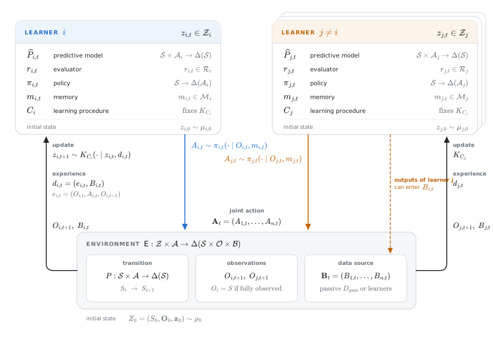
Conditional on the joint action, the environment supplies a successor state, observations, and incoming batches. Each learner then updates from their received experience. For finite spaces, multiply the conditionally independent update probabilities and sum over the possible batches. With \(e_i=(o_i,a_i,o_i')\), this gives the system transition kernel \(P^{\mathrm{sys}}\)

\[ P^{\mathrm{sys}}(Z'\mid Z,\mathbf a) =\sum_{\mathbf B}\mathsf E(s',\mathbf o',\mathbf B\mid Z,\mathbf a) \prod_i K_i\bigl(z_i'\mid z_i,(e_i,B_i)\bigr) \]

A joint update kernel replaces the product for shared update randomness (for continuous variables, we can use integrals). If there’s no incoming data, the sum uses only \(\mathbf B=([],\ldots,[])\) and we recover the interaction-only construction.

The time index counts events in the specified process. Physical actions, completed trials, comparison reports, and evaluator revisions need not occur together. Clocks and the current phase belong in the state; unfinished trials and retained comparisons belong in memory. Components remain unchanged at events that do not update them. If one agent’s revision affects the next reported preference, those events must occur in order, rather than being treated as simultaneous updates from the same prior state.

Death and replacement are also rules of the environment. With a fixed number of slots, the state records whether each slot is occupied and which individual occupies it. An inactive slot has only a no-op action, and its learner state remains unchanged until replacement. A replacement rule specifies the newborn’s physical state, learner initialization, and any inheritance. We represent this by an environment reset kernel \(L(dZ'\mid\widetilde Z)\), applied after the ordinary transition:

\[ (L\circ P^{\mathrm{sys}})(dZ'\mid Z,\mathbf a) =\int L(dZ'\mid\widetilde Z)\, P^{\mathrm{sys}}(d\widetilde Z\mid Z,\mathbf a) \]

Where replacement is enabled, use this composed transition for \(P^{\mathrm{sys}}\) in subsequent rollouts. Other event orders must likewise be specified. Copying a survivor’s evaluator into a newborn can change its prevalence without any surviving agent revising its evaluator.

Write \(\pi_i(a\mid Z)\) for the action distribution of learner \(i\) in state \(Z\). Policies may change as \(Z\) evolves. Under independent action selection, forcing agent \(i\)’s present action to \(a\) gives

\[ P_i^{\pi}(Z'\mid Z,a) =\sum_{\mathbf a_{-i}} \left[\prod_{j\neq i}\pi_j(a_j\mid Z)\right] P^{\mathrm{sys}}(Z'\mid Z,(a,\mathbf a_{-i})) \]

This intervention leaves the other agents’ current action rules intact and then lets every learner continue updating. A rollout (a simulated continuation from a specified system state) must therefore retain the learners’ memories, evaluators, policies, and relevant shared records, as well as the environment state.

Evaluating a Developing Learner

The learning loop specifies how the learner acts and changes. We now ask how to compare possible actions when their consequences include changes to the learner’s own evaluator. By specifying which evaluator scores each continuation, we can derive an action value and a Bellman recursion while allowing the learner to keep learning.

Fix a bounded evaluator \(r\). During the rollout, every learner continues to update according to their procedure, including changes to their evaluator and policy. The fixed \(r\) assesses that development.

For joint-action consequences, define the record

\[ X_{i,t+1}=(S_t,\mathbf A_t,S_{t+1}) \in\mathcal S\times\mathcal A\times\mathcal S \]

Here \(\mathcal A=\prod_j\mathcal A_j\), and \(r:\mathcal S\times\mathcal A\times\mathcal S\to\mathbb R\). The earlier own-action evaluator is the restriction \(r(s,\mathbf a,s')=\widetilde r(s,a_i,s')\). The consequence record specifies what the evaluator assesses. The observation component of \(\mathsf E\) determines what information the learner receives.

For the additive scoring rule, a trajectory \(\tau\) of the full system, and \(0\leq\gamma<1\), define

\[ G_r(\tau)=\sum_{k\geq0}\gamma^k r(X_{i,k+1}) \]

The continuation behavior \(\pi\) is generated by the evolving learner states. Under the intervention above, the action value is

\[ Q_r^{\pi}(Z,a) =\mathbb E^{a,\pi}\left[ \sum_{k=0}^{\infty}\gamma^k r(X_{i,k+1}) \mid Z_0=Z \right] \]

Splitting \(G_r\) into the first assessment and discounted remainder and taking expectations gives

\[ \begin{aligned} Q_r^{\pi}(Z,a) &=\mathbb E\left[ r(X_{i,1})+\gamma V_r^{\pi}(Z_1) \mid Z_0=Z,\operatorname{do}(A_{i,0}=a) \right]\\ V_r^{\pi}(Z) &=\sum_a\pi_i(a\mid Z)Q_r^{\pi}(Z,a) \end{aligned} \]

This is Bellman policy evaluation on the full system state \(Z\), including the environment and learner states. Replacing the fixed evaluator used to compute the return with the future actor’s evaluator would evaluate a different return. We use \(\widehat Q\) for an estimate under a learned model; under partial information, that model also supplies a distribution over possible system states at the decision time.

Comparing Possible Developments

Different experiences may produce evaluators that disagree about the same decision. We compare their assessments of each available action to make that disagreement explicit. The comparison supplies information for a learning procedure without specifying which evaluator the learner should adopt.

Let \(r_b\) be the evaluator obtained after simulated learning trajectory \(b\). At horizon \(H\), evaluate every candidate initial action under each resulting evaluator:

\[ M_{ba}=Q_{r_b,H}^{\pi}(Z,a) \]

Each row contains action values under one evaluator; each column contains values of one action under different evaluators. Include the present evaluator as row \(0\). With \(m\) independently sampled consequence trajectories per action,

\[ \widehat M_{ba} =\frac1m\sum_{\ell=1}^m\sum_{k=0}^{H-1} \gamma^k r_b\bigl(X_{i,k+1}^{a,\ell}\bigr) \]

Fix copies of the resulting evaluators, then draw fresh trajectories for them to assess. Reusing the trajectories that produced those evaluators could bias the comparison in their favor. These estimates still depend on the accuracy of the predictive model. If \(|r(x)|\leq R_{\max}\), stopping the return calculation after \(H\) steps introduces an error of at most \(R_{\max}\gamma^H/(1-\gamma)\). For the action \(a_0\) taken,

\[ \operatorname{Regret}_{r_b}(a_0) =\max_a M_{ba}-M_{ba_0} \]

The learner can select the action with the highest value under their current evaluator, while retaining the other evaluators’ assessments as evidence for revision. Choosing or combining evaluators remains a decision-rule choice.

The relation \(\mathcal I(h,h')\) specifies which developments count as continuations of the actor. This relation may depend on retained memory, which earlier learner a copy came from, and constraints on revision, without requiring identical preferences. Copies treated as distinct agents can still supply social evidence.

Reevaluating Earlier Experience

Revising the evaluator may change the scores assigned to past experience. We derive the change in return when the recorded events remain fixed and only the evaluator changes.

For retained transition records \(x_u,\ldots,x_{T-1}\), evaluated at time \(t\geq T\), define

\[ G_{u:T}^{[t]} =\sum_{k=u}^{T-1}\gamma^{k-u}r_t(x_k) \]

Holding the records fixed while revising the evaluator gives

\[ \boxed{ G_{u:T}^{[t+1]}-G_{u:T}^{[t]} =\sum_{k=u}^{T-1}\gamma^{k-u} \left[r_{t+1}(x_k)-r_t(x_k)\right] } \]

Let \(\Delta r_u=r_{t+1}(x_u)-r_t(x_u)\) and \(\Delta G_u=G_{u:T}^{[t+1]}-G_{u:T}^{[t]}\). The change propagates backward:

\[ \begin{aligned} \Delta G_T&=0\\ \Delta G_u&=\Delta r_u+\gamma\Delta G_{u+1} \end{aligned} \]

This derives retrospective reevaluation without new facts about the past. Some changes may cancel. The memory must retain records sufficient for the revised evaluator: old scores alone generally do not suffice, and learned value estimates need rescoring or replay. Assessing whether the earlier choice was mistaken additionally requires counterfactual continuations from the system state before the earlier choice, evaluated under the chosen reward model.

Learning from Other Agents’ Trajectories

Other agents may have experienced outcomes the learner has not. We establish when their trajectories can inform the learner’s counterfactual estimates, and why sharing their scores alone may be insufficient for evaluation under the learner’s own evaluator.

A peer’s trajectory can provide evidence about what would have happened had the learner taken action \(a\). This requires equality of the following probabilities for every measurable set \(D\) of trajectories:

\[ \Pr(\tau_i^a\in D\mid c_i) =\Pr\bigl(\mathcal T_{j\to i}(\tau_j)\in D\mid A_j=a,c_j\bigr) \]

where \(c_i,c_j\) record the relevant contexts and \(\mathcal T_{j\to i}\) translates the source’s trajectory description. Establishing this equality requires comparable circumstances, observations of the actions being compared, and accounting for why the observed agents chose those actions. Observing a peer alone does not establish it.

The source’s reported reward is also generally insufficient to reconstruct the learner’s reward. For two models on a common domain of transition records, a function satisfying

\[ r_i(x)=f\bigl(r_j(x)\bigr) \]

exists when

\[ r_j(x)=r_j(y) \;\Longrightarrow\; r_i(x)=r_i(y) \]

Necessity follows because \(f\) cannot distinguish equal inputs. For sufficiency, assign each source score the target score of any record producing it; the implication makes the assignment well-defined. If the condition fails, the source has discarded a distinction the learner needs. Transmitting the transition or trajectory allows the same experience to be evaluated under another reward model.

The appendix gives the table of related learning methods and derivations connecting this framework to familiar learning problems and update rules.

In this section, I’ll explore Social CartPole, a Social Learning environment based on CartPole (a standard RL environment). Subsequent works can try different environments, but are out of scope.

Standard CartPole

Let’s start by examining the well-known CartPole environment; subsequent sections will introduce more and more social mechanisms.

In standard CartPole, an agent learns to push a cart left or right to keep a hinged pole upright. At each stage, the agent observes four quantities:

cart position \(x\)
cart velocity \(v\)
pole angle \(\theta\)
angular velocity \(\omega\)

Together, these form the state \(s=(x,v,\theta,\omega)\). We write \(S_t\) for the state observed at time \(t\). The action \(a\) is a horizontal force applied to the cart for 0.02 seconds. Writing \(F(a)\) for that force:

\[ F(a)= \begin{cases} -10\,\mathrm N & a=\text{left}\\ +10\,\mathrm N & a=\text{right} \end{cases} \]

The simulator uses this force and the current state to update the cart’s position and velocity and the pole’s angle and angular velocity. The agent then observes the new state and chooses its next push.

In the standard CartPole, the agent receives a reward of one at each step. The episode ends immediately if

the pole tilts too far (> twelve degrees)
the cart leaves the track

Maximizing accumulated reward therefore encourages balancing.

In this work, we will examine a few different learning methods orthogonal to the question of social learning. Each method connects an evaluator to a method for choosing actions. We begin with the supplied CartPole reward, then ask whether agents can fit evaluators to another agent’s reported comparisons, and whether peer interaction can revise those evaluators to support useful behavior.

Note: Each method may use slightly different environments, representations, and budgets. The goal is to demonstrate social learning across different methods for choosing actions.

Each method specifies how the learning procedure \(C_i\) chooses or improves actions. As above, learner \(i\) at update event \(t\) has a state \(z_{i,t}\) containing a predictive model \(\widehat P_{i,t}\), evaluator \(r_{i,t}\), policy \(\pi_{i,t}\), learning procedure \(C_i\), and memory \(m_{i,t}\):

\[ z_{i,t}=(\widehat P_{i,t},r_{i,t},\pi_{i,t},C_i,m_{i,t}) \]

A trial record \(\tau\) contains the states and actions of a performance; \(G_{r_{i,t}}(\tau)\) is its score under the current evaluator. The expectation \(\mathbb E_{P,\pi}\) averages over the trials generated by the environment \(P\) and the policy \(\pi\). If we hold the evaluator fixed, the control objective is

\[ \max_\pi\ \mathbb E_{P,\pi}\!\left[G_{r_{i,t}}(\tau)\right] \]

For a finite performance, the sum defining \(G_r(\tau)\) ends at the last recorded transition. Undiscounted sums use \(\gamma=1\).

Below, we suppress the agent index \(i\). The environment follows \(P\); a dynamics model \(\widehat P_t\) predicts the next state from the current state and action. Each control update uses a fixed evaluator \(r_t\). Reported comparisons arrive as incoming data \(B_t\) and can revise \(r_t\) between updates. Trial records and other retained learning state belong to \(m_t\).

Also, for policies with weights, \(\pi^w\) denotes the policy with weight vector \(w\), and \(w_t\) contains the current weights. A candidate policy \(\pi'\) produces a trial \(\tau_{\pi'}\). A finite candidate set is denoted \(\Pi_t\), \(\arg\max\) denotes the candidates attaining the highest score, and \(\pi^\star\) denotes a selected candidate.

Let us now review the training mechanisms (click on one and all of the related cards will swap throughout the report).

Proximal Policy Optimization (PPO) is a policy-gradient method. PPO collects trajectories using the current policy \(\pi_t\), then updates the policy weights to increase expected return. The policy \(\pi_t(a\mid s)\) gives the probability of pushing left or right in state \(s\).

A learned value function, called the critic, estimates \(V_{r_t}^{\pi_t}(s)\), the expected return from \(s\). The action value \(Q_{r_t}^{\pi_t}(s,a)\) is the expected return from taking \(a\) and then following \(\pi_t\). Their difference is the advantage \(A_{r_t}^{\pi_t}(s,a)\)

\[ A_{r_t}^{\pi_t}(s,a) =Q_{r_t}^{\pi_t}(s,a)-V_{r_t}^{\pi_t}(s) \]

Let \(k\) index transitions in the collected batch, with state \(s_k\) and action \(a_k\). Rewards and the critic provide an advantage estimate \(\widehat A_k\). Positive advantages favor increasing an action’s probability; negative advantages favor decreasing it.

For candidate weights \(w\), define the probability ratio \(\rho_k(w)\) relative to the policy that collected the batch

\[ \rho_k(w)=\frac{\pi^w(a_k\mid s_k)}{\pi_t(a_k\mid s_k)} \]

PPO-Clip maximizes the objective \(L_t(w)\). Here \(\epsilon>0\) is the clipping width, \(\operatorname{clip}_{1-\epsilon}^{1+\epsilon}\) truncates a ratio to that interval, and \(\mathbb E_k\) averages over the batch

\[ L_t(w)=\mathbb E_k\!\left[ \min\! \begin{Bmatrix} \rho_k(w)\widehat A_k\\ \operatorname{clip}_{1-\epsilon}^{1+\epsilon}\!\bigl(\rho_k(w)\bigr)\widehat A_k \end{Bmatrix} \right] \]

Starting at \(w_t\), several gradient-ascent steps give \(w_{t+1}\) and the updated policy

\[ \pi_{t+1}=\pi^{w_{t+1}} \]

Clipping removes the incentive to change an action’s probability too far on the same batch. The critic is fitted to estimated returns, then the updated policy collects the next batch.¹⁴

¹⁴ See OpenAI’s PPO explanation, the value-function definitions, and the original PPO paper.

Our smallest controller takes a weighted sum of the four observations and adds a bias. A sigmoid turns the result into a probability of pushing right. PPO learns these five parameters from the rewards received during training.

Randomly initialized PPO policies were trained with the standard reward of one point per step.

Experiment Details

Eight policies were trained independently, each for 100,096 simulated pushes. Each policy had four observation weights and a bias. The critic used eight tanh hidden units to estimate returns. Each trained policy was tested from 100 fresh starts close to upright and 100 starts tilted six to ten degrees, choosing the more likely push at each step. Another 100 near-upright tests per policy used sampled pushes. Tests lasted ten seconds. The cart and pole had to remain within the failure boundaries, and the root-mean-square pole angle over the final five seconds was also measured.

Before training, none of the controllers balanced for ten seconds from the tested near-upright starts. After training, every controller balanced from every tested near-upright and tilted start. Sampling pushes also gave ten seconds of balancing in every test. In every trained-policy test, the root-mean-square pole angle over the final five seconds was below five degrees.

Direct policy search evaluates candidate policies by running them in the environment and comparing their returns. In this track, each round tests a population of controllers, including existing controllers, mutations, and new random controllers.

For the first three experiments, let \(\Pi_t\) be the candidate population, \(M\) the number of starting states, and \(\tau_{\pi'}^{(j)}\) the trajectory produced by candidate \(\pi'\) from start \(j\). Each candidate is tested from the same starts. Selecting the highest average return gives

\[ \pi_{t+1}\in\underset{\pi'\in\Pi_t}{\arg\max} \frac{1}{M}\sum_{j=1}^{M}G_{r_t}\!\left(\tau_{\pi'}^{(j)}\right) \]

The controllers were trained with the standard reward of one point per step. The final policies were then tested from fresh starting states, with ten seconds of balancing required in each test.

Experiment Details

Sixty recurrent controllers were evaluated in each search round. The candidates comprised twelve current controllers, three mutations of each, and twelve newly initialized controllers. Every candidate was tested from the same four starting states. A highest-scoring candidate was selected with 90% probability and a random candidate otherwise.

Eight development populations were followed by eight fresh confirmation populations. Each was trained for forty rounds. The twelve final controllers in each population were tested from twenty starts close to upright and twenty leaning starts each.

From starts close to upright, the cart and pole stayed within the failure limits in 28 of 1,920 tests before training and 1,828 afterward, or 1.5% and 95.2%. Every trained population succeeded in at least 88.3% of these tests. From leaning starts, the corresponding result was 1,541 of 1,920 tests, or 80.3%.

Before training, the controllers kept the pole balanced for ten seconds in fewer than 2% of tests starting close to upright. After training, balancing succeeded in 95% of these tests. From larger initial tilts, balancing lasted ten seconds in 80% of tests. Performance varied across the independently trained populations.

Stochastic hill climbing changes the current policy by a random perturbation, tests the candidate, and keeps the change if the score improves. For current weights \(w_t\) and a random perturbation \(\Delta w\), the candidate policy is

\[ \pi'=\pi^{w_t+\Delta w} \]

Run \(\pi'\) to obtain a trial \(\tau_{\pi'}\) and score the trial with \(G_{r_t}\). Let \(\overline G_t\) be the estimated score of the current policy. The update is

\[ \pi_{t+1}= \begin{cases} \pi' & G_{r_t}(\tau_{\pi'})>\overline G_t\\ \pi_t & G_{r_t}(\tau_{\pi'})\leq\overline G_t \end{cases} \]

A linear policy was used to choose each push. The four scaled observations were multiplied by four weights and added to a bias; the sign of the sum determined the direction.

At each update, the current and proposed policies were tested from the same eight fresh starting states. Rewards were summed across the eight episodes, and the proposal was accepted when its total was higher. Training used the standard reward of one point per step, with episodes ending at failure or after 500 steps (ten seconds).

Experiment Details

Each controller was trained with a budget of 960,000 simulated pushes, counting the evaluations of both current and proposed policies. The policy weights were normalized after each proposal. Gaussian perturbations cycled through standard deviations of 0.05, 0.15, 0.5 and 1.5.

Eight independently trained controllers were each tested from 100 fresh close-to-upright starts and 100 starts initialized with a lean of six to ten degrees. The cart and pole stayed within the failure limits for ten seconds in all 800 close-to-upright tests and 667 of the 800 leaning tests, or 83.4%.

Training produced controllers that kept the pole balanced for ten seconds from every tested start close to upright. A larger initial tilt made the task harder, but balancing still lasted the full ten seconds in 83% of those tests.

The above experiments establish that, with a suitable reward supplied, our learner can acquire the desired behavior.

Changing the Reward

So we know (based on the above) that given the reward, we can make the agent balance the pole. Can we adjust where they end up balancing the pole? Let’s look at a (somewhat toy) example.

Let \(\theta'\) be the angle after the action. The twelve-degree cutoff gives an angular scale:

\[ \theta_c=12\frac{\pi}{180}\approx0.20944 \]

So a different reward should select where the pole is balanced. Let \(x_*\) be the target position, either one metre left of centre or one metre right. For the next state \(s'=(x',v',\theta',\omega')\), we supplied the reward

\[ r_{x_*}(s,a,s')=\exp\left[-(x'-x_*)^2-\left(\frac{\theta'}{0.20944}\right)^2-0.1(v')^2-0.01(\omega')^2\right] \]

\[ x_*\in\{-1,+1\} \]

Positions are measured in metres, angles in radians, and time in seconds. The terms favor the target position, uprightness, and low linear and angular speed. Only the target position was changed between conditions. Physics, controller architecture, initialization, starting-state generator, and computational budget were matched within each method.

Both controllers were shown from the same centre start. Survival was assessed over twenty seconds in CartPole, with failure beyond 2.4 metres from centre or twelve degrees from upright. Fresh test states were drawn with each coordinate independently uniform on \([-0.05,0.05]\). Target holding additionally required every state in the final ten seconds to remain within 0.15 metres of the target, with speed at most 0.25 metres per second and angle at most five degrees.

Separate policies were trained to balance at the left and right targets using PPO. Each policy represented the probability of pushing right with four observation weights and a bias. These parameters were updated using the supplied target reward. The primary evaluation selected the more likely push at each step. A separate evaluation sampled pushes according to the same policy probabilities.

Experiment Details

Eight initial policies were each copied into a left-target and a right-target condition. The initial critic parameters, procedure for generating starting states and budget of 1,000,192 simulated pushes were the same within each pair. Each trained controller was tested from the exact centre and from 100 fresh starting states for twenty seconds. Both ways of choosing pushes were evaluated on the same controllers. Success required completing the test and, at every step of the final ten seconds, staying within 15 centimetres of the target, below or at 0.25 metres per second in speed, and within five degrees of upright. The deterministic primary evaluation and the separate sampled-action evaluation were specified before training.

Sampling pushes from the same policies also kept every pole balanced for twenty seconds. In all 1,600 fresh-start tests, the cart stayed within the target-position and pole-angle tolerances throughout the final ten seconds. Brief excursions above the speed limit reduced the full-criterion pass rate to 21.8% at the left target and 16.5% at the right. Among failed tests, the median total time above the speed limit was 0.04 seconds.

Choosing the more likely push at each step, PPO reached and held both targets in every test. All eight policies per target succeeded from all 100 fresh starts and from the exact centre.

Populations of recurrent controllers were trained separately under the two target rewards. Each controller mapped the observed state and recent actions to a push direction. Candidates were ranked by the total reward over their performances. High-scoring controllers were retained and mutated, and newly initialized candidates were added in each search round.

Experiment Details

Eight initial populations were each copied into a left-target and a right-target condition. Training consisted of forty search rounds, with sixty candidates evaluated from the same four starting states in each round. Training episodes lasted up to twenty seconds. All twelve final controllers in each population were evaluated.

All twelve final controllers from each of eight populations were evaluated, giving 9,600 fresh tests per target. The target-holding criterion was met in 1,045 left-target tests and 2,621 right-target tests, or 10.9% and 27.3%.

The cart and pole stayed within the failure limits for twenty seconds in 8,799 left-target tests and 8,867 right-target tests, or 91.7% and 92.4%.

Most controllers could keep the pole balanced for twenty seconds, but reaching and staying at the requested location was much less reliable. The left target was held in about 11% of tests and the right target in about 27%. This training budget usually produced survival without the requested position control.

Separate linear controllers were trained to balance at the left and right targets. The four observation weights and bias were perturbed, and the current and proposed controllers were evaluated from the same starting states. A proposed change was retained when the summed target reward increased. The same training procedure and budget were used for both target locations.

Experiment Details

For each policy update, the current and proposed controllers were tested from the same eight fresh starts for up to twenty seconds.

A separate experiment tested whether additional training improved settling at the target. Eight new initial policies were each trained toward both targets and evaluated after 3,840,000 and 15,360,000 simulated pushes. The longer training continued the same searches, with unchanged proposal sizes and starting-state procedures. Each resulting controller was tested from the exact centre and from 100 fresh starting states.

With the shorter budget, the left target was reached and held in 58.5% of fresh tests and the right target in 67.9%. With the longer budget, these rates were 98.6% and 94.4%. The cart and pole remained within the failure limits for twenty seconds in 98.6% of left-target tests and every right-target test under the longer budget.

Before training, further confirmation was made conditional on at least 90% average target holding on each side, at least 80% for every controller, and successful holding from the exact centre by every controller. The weakest right-target controller reached 55% on fresh starts, so the criterion was not met and further confirmation was not run.

All sixteen trained controllers moved from the centre to the location specified by the reward and balanced there. Across fresh starting states, the left target was reached and held in 98.6% of tests and the right target in 94.4%.

Changing the supplied reward selected different surviving behaviors. Controllers learned to balance one metre left or right of centre.

Note: Given that an agent survives and holds a static equilibrium, we can think of the locations as giving an equivalence class of possible solutions (dynamic equilibria are also possible).

Learning a Reward With a Teacher

Changing the reward changes what the controller learns to do. But we still directly programmed that reward into a specific agent. Instead, can an agent learn rewards from information about what someone else prefers?

To test this, a teacher whose evaluator favored uprightness was used to label pairs of performances. Each learner received the records and the label, then revised its evaluator based on these comparisons. Changes in the learner’s rankings were measured against the teacher’s, and the revised evaluator was used to guide policy learning. The resulting balancing behavior was measured separately.

The learner’s reward was represented by two coefficients

\[ r(s,a,s')=b+c u^2 \]

Here \(u=\tanh(\theta'/0.20944)\) is the bounded next-state angle. Both \(b\) and \(c\) were learned from comparisons. The teacher used \(1-u^2\) to score performances and supplied only the comparison labels.

The teacher favored uprightness while penalizing displacement and velocity. The teacher score per step was \(\cos(\theta)-0.1\tanh^2(x/2.4)-0.01\tanh^2(v/3)\). Learners received only the resulting comparison labels. Cart travel and pole rotation were unrestricted in this experiment.

To learn a reward from the teacher comparisons, the learner’s evaluator was represented by a neural network and fitted to the comparison labels. A separate policy network mapped the cart and pole observations to the probability of pushing right. The policy was trained with PPO using rewards from the learned evaluator, with a third network estimating returns as the critic. Evaluator fitting and policy training were alternated. The evaluator was then held fixed for a final period of policy training.

Experiment Details

The actor, critic and evaluator each had five inputs, eight tanh hidden units and one output, giving 57 parameters per network. The observations were tanh-scaled position, velocity and angular velocity, together with the sine and cosine of the pole angle. The actor used a sigmoid output for action probabilities. The evaluator used a tanh output for bounded rewards.

Training episodes lasted four seconds with unrestricted cart travel and pole rotation. Five populations of six learners were run per condition. Three learners were replaced after the twelfth of sixteen social rounds. Each continuing learner received 131,072 policy-training transitions followed by 32,768 transitions with the final evaluator fixed.

Each learner received eight comparisons per round and retained the latest 64. Evaluator fitting used a logistic comparison loss with a penalty for changing previous scores. The control retained random private evaluators. The final test measured whether the root-mean-square wrapped pole angle stayed below five degrees over the last five seconds of a ten-second performance.

In this PPO experiment, cart travel and pole rotation were unrestricted. Success required the root-mean-square wrapped pole angle to remain below five degrees over the final five seconds of a ten-second test. Learning from teacher comparisons raised success from 1.0% to 50.3%. In separate comparisons of postures, 76.7% of the learned evaluators preferred uprightness.

To learn a reward from the teacher comparisons, a reward model with two coefficients was fitted to the comparison labels. The learned reward was then held fixed while a population of recurrent controllers was trained by direct policy search. Each candidate was evaluated by summing the learned reward over the resulting performance. High-scoring controllers were retained and mutated to produce candidates for the next round.

Experiment Details

For each training dataset, 64 performances were recorded from randomly initialized controllers and used to form 512 comparisons. Half compared whole performances, allowing duration to affect the teacher’s choice. Half compared excerpts of equal length, allowing the effect of tilt to be distinguished from duration.

With labels withheld, the initial random reward was retained. A second control reversed every label. In the treatment, the teacher labels were retained. All three conditions used the same performance pairs. The fitted coefficients were held fixed while control was learned or planned.

Eight independently generated comparison datasets were used. For each dataset, control was evaluated with the initial random reward, the reward fitted to reversed labels, and the reward fitted to teacher labels.

For each of the eight comparison datasets, a population of recurrent controllers was trained for forty search rounds. Each round evaluated twelve current controllers, thirty-six mutations and twelve newly initialized candidates. The initial controllers, starting states and number of search rounds were the same across the three reward conditions.

Balancing required ten seconds within the standard rail and pole-angle limits. The root-mean-square pole angle also had to be below five degrees over the final five seconds.

Each of eight populations contributed twelve final controllers, each tested from twenty starts close to upright and twenty leaning starts. For starts close to upright, 20 of 1,920 tests met the requirement without labels, zero with reversed labels and 1,840 with teacher comparisons. These rates were 1.0%, 0% and 95.8%.

From leaning starts, the corresponding counts were 30, zero and 1,769, or 1.6%, 0% and 92.1%.

With teacher labels withheld, balancing was rare. With labels reversed, no test met the balancing requirement. With accurate teacher comparisons, the controllers stayed upright for ten seconds in about 96% of tests starting close to upright and 92% starting at a larger tilt. Relative to the controls, every paired population benefited from the teacher comparisons.

To learn a reward from the teacher comparisons, a reward model with two coefficients was fitted to the comparison labels. The learned reward was then held fixed while a new linear controller was trained by stochastic hill climbing. The four observation weights and bias were perturbed, and the current and proposed controllers were tested from the same starts. A proposal was retained when the summed learned reward increased.

Experiment Details

Each controller was initialized independently of the teacher. Policy updates were evaluated by comparing the summed reward over whole episodes.

Training episodes lasted up to forty seconds, allowing slow cart drift to reach the rail and affect the return. At each update, the current and proposed controllers were tested from the same four starts close to upright and four leaning starts. Each training run used a budget of 15,360,000 simulated pushes. The proposal schedule included perturbation sizes of 0.005 and 0.015 as well as 0.05, 0.15, 0.5 and 1.5. These settings were the same across all three label conditions. Final tests lasted ten seconds.

Balancing required ten seconds within the standard rail and pole-angle limits. The root-mean-square pole angle also had to be below five degrees over the final five seconds.

Sixteen fresh confirmation runs were each tested from 100 starts close to upright and 100 leaning starts. Without labels, 661 of 1,600 tests close to upright met the balancing requirement, or 41.3%. With reversed labels, none did. With teacher comparisons, all 1,600 tests of each kind met the requirement.

For each comparison, the feature vectors were summed over each performance and their difference was used to fit a logistic model to the teacher’s label. Feature differences were scaled by their root-mean-square values across the training comparisons. Fitting used L2 regularization of 0.001 and forty Newton iterations with backtracking. Before policy learning, the coefficients were converted to the original feature scale and divided by a positive normalization constant. Agreement with the teacher on separate, unused comparisons was 94.5%. The training procedure was selected using eight development runs and then fixed for sixteen independent confirmation runs. Settings and results for every run are available.

Without labels, balancing succeeded in about 41% of near-upright tests. With reversed labels, success was zero. With accurate teacher comparisons, the controllers kept the pole upright for ten seconds in every test, including initial tilts of six to ten degrees.

The comparisons carried information about how performances were evaluated, and the learned evaluator then guided behavior.

Learning a Reward Without a Teacher

In the above experiments, balancing gives us an outcome we can recognize without much interpretation. We’ve established that where balancing occurs, and how the object moves, may vary. However, all the above experiments involve putting the reward in somewhere. Can we induce “uprightness” preferences in the agents without actually giving them rewards a priori?

In particular, in the last experiment the teacher supplied a fixed preference for uprightness. The next question is whether useful evaluators can develop through interaction among peers.

A source with an upright-valuing reward supplies the preference ordering we hoped to explain. We now remove that source and let agents report pairwise preferences using their own evaluators. Can these reports revise the evaluators to support recognizable behavior without a supplied target reward?

One possibility is to start with agents that have no preferences at all (or rather, random preferences). Unfortunately, this immediately exposes a problem with the update rule. If every evaluator is zero, every performance receives the same score. Nobody expresses a strict preference, so nobody receives information that would change their evaluator. More exploration does not break this symmetry.

Agents were therefore initialized with different, randomly drawn evaluators. Each agent used their current evaluator to compare their own performance to a peer’s performance, then sent the comparison label to that peer. The receiving agent revised their evaluator using the comparisons they received and used the revised evaluator to guide control. No agent was assigned a fixed reward that the rest of the population was meant to acquire.

A revision could change how an agent acted, changing what other agents subsequently observed and compared. To test whether this interaction helped control, matched populations were trained with evaluator revision disabled or enabled. The control populations retained their private evaluators, allowing the contribution of peer comparisons to be assessed. Balancing was measured in fresh tests. The test criterion was not supplied as a training reward.

Each learner controlled a separate cart. A physical performance ended after four seconds or when the cart or pole crossed a failure boundary. The cart and pole were reset between performances, and learning continued across those performances.

Peer sampling was deliberately subject to inspection bias. At each observation, a source was chosen uniformly from the agents currently performing. After a fall, an agent spent one second recovering and could not be selected as a source. Agents that fell frequently spent more time unavailable. Agents that continued performing spent more time in the source pool and had more opportunities to be observed.

This gave physical persistence a route into evaluator learning. An evaluator that supported longer performances could supply more of the comparison labels used to revise other evaluators. The same source also supplied examples of control that other agents could copy. We tested whether this feedback could turn initially random evaluators into rewards that supported balancing.

Balancing was assessed in eight-second tests from fresh starts close to upright and from starts tilted six to ten degrees. The cart and pole had to remain within the failure boundaries throughout. The root-mean-square pole angle over the final four seconds also had to be below five degrees.

A weighted sum of the four scaled observations and a bias determined the probability of pushing right. Actions were sampled from this policy, and PPO used the resulting trials to update the five policy parameters. A linear critic estimated returns. Controllers fitted to observed peer performances could also be tried and adopted according to the learner’s evaluator. PPO updates used trials collected by the current policy.

Experiment Details

The experiment was repeated sixteen times. Each run compared two groups of 32 agents over eighty simulated minutes. One group kept the initial evaluators fixed, while the other revised them using peer comparisons of whole performances. Evaluators began with random preferences for regions of the physical state space. Agents recovered for one second after failure. Policy copying was enabled in both groups, and every agent was retained.

The five policy inputs were \(\sin(\theta)/0.2\), \(\omega/2\), \(v/2\), \(x/2.4\) and a constant input of one. During training, pushes were sampled from the policy. On cycles used for PPO updates, the policy collected experience over two successive five-second trials. PPO updates used those sampled-policy trials. Controllers fitted from observed peer performances were evaluated on separate copying cycles.

Each controller was tested from twelve fresh starts close to upright and twelve tilted starts, with 5% motor noise. Both the more likely push and sampled pushes were evaluated.

With private evaluators, balancing succeeded in 21.5% of tests starting close to upright when the more likely push was chosen. With peer comparisons, success rose to 50.6%. From tilted starts, private evaluators gave 19.4% success and peer comparisons gave 46.9%. With sampled pushes, private evaluators gave 16.3% near-start success and peer comparisons gave 39.5%. From tilted starts, private evaluators gave 13.5% and peer comparisons gave 32.0%.

The near-start improvement occurred in eleven of sixteen population pairs under either test procedure. No successful upright tests were obtained in five of the populations trained with peer comparisons, so the improvement was not universal; however, this shows that it is possible to learn a reward starting from “random” rewards and social learning (note that there is inspection bias in peer sampling by design).

Each learner searched a bank of linear controllers. A controller selected pushes from a weighted sum of the four scaled observations and a bias. Candidates were tried sequentially and ranked by the learner’s current evaluator. High-scoring candidates supplied parents for mutations, while new random controllers and controllers fitted to peer performances supplied further proposals.

Experiment Details

Each learner maintained sixty controllers. The five policy inputs were \(\sin(\theta)/0.2\), \(\omega/2\), \(v/2\), \(x/2.4\) and a constant input of one. Candidates were tested sequentially in five-second trials, beginning from the current physical state. Stored trajectory features were scored under the current evaluator. The best twelve controllers became parents for thirty-six mutations and twelve newly initialized candidates. When a controller fitted from a peer performance was available, a copied controller was selected with 50% probability for the proposal trial.

Each controller was tested from twelve fresh starts close to upright and twelve tilted starts, with 5% motor noise. Four populations trained with peer comparisons produced no successful balancing tests.

With private evaluators, balancing succeeded in 13.6% of tests starting close to upright. With peer comparisons, success rose to 34.5%. From tilted starts, private evaluators gave 9.6% success and peer comparisons gave 26.2%. Relative to private evaluators, twelve of the sixteen populations benefited from peer comparisons.

Population learning used randomly initialized evaluators and sequential five-second policy trials. A trial was scored from all motion during that interval, which could span several physical performances. Each new trial began from the then-current physical state.

Each learner proposed changes to a linear controller and retained proposals whose scores exceeded the stored score for the current policy. Half the proposals were fitted from observed peer performances when those records were available. The remaining proposals were random changes to the policy weights. The current evaluator scored both kinds of proposal.

Experiment Details

To test whether peer comparisons improved control without a teacher, populations were initialized with random evaluators and trained with evaluator revision either disabled or enabled. For an exchange from Agent A to Agent B, Agent A scored A’s last completed performance and B’s last completed performance using A’s reward function. Agent B received the performance records and a label identifying which performance A scored higher. Agent B revised B’s reward function using the eight most recent comparisons B had received. Physical, temporal, and local state-space features were included, with no assigned uprightness bonus.

Performances were started near upright and ended after four seconds, at a twelve-degree pole angle, or when the cart left the track. The cart and pole were then reset near upright, immediately after success or after one second of recovery following failure. Scores were summed over performing moments, including a learned constant term. A positive constant could therefore favor continuing, while a negative constant could favor ending.

Balancing was tested for eight seconds from fresh starting states. The cart had to stay on the track and the pole within the failure angle throughout. The root-mean-square pole angle also had to be below five degrees over the final four seconds. This criterion was applied during evaluation.

The experiment was repeated sixteen times. Each run compared two groups of 32 agents over eighty simulated minutes. One group kept the initial evaluators fixed, while the other revised them using peer comparisons. Policy copying was enabled in both groups, and every agent was retained. Relative to private evaluators, peer comparisons improved balancing by a mean of 35.8 percentage points. Resampling whole population pairs gave a 95% interval from 24.2 to 45.9 points. Two populations trained with peer comparisons produced no successful balancing tests.

With private evaluators, balancing succeeded in 17.7% of tests starting close to upright. With peer comparisons, success rose to 53.5%. From tilted starts, private evaluators gave 13.3% success and peer comparisons gave 44.4%. Relative to private evaluators, fourteen of the sixteen populations benefited from peer comparisons.

The experiment was also repeated sixteen times with policy copying disabled. Each run compared two groups of 32 agents over eighty simulated minutes, one with fixed evaluators and one with evaluators revised from peer comparisons. No agents died. All active-trial transitions were retained when calculating policy scores. With private evaluators, near-start upright success was 7.3%, compared with 17.4% with peer comparisons. From leaning starts, the rates were 6.3% with private evaluators and 14.4% with peer comparisons.

Relative to private evaluators, peer comparisons improved balancing under the sequential-trial procedure with policy copying disabled and every agent retained.

The replay below follows the 32-agent population with policy copying disabled during training. Each arrow runs from the agent sending a preference to the agent receiving that preference. Select an exchange to see the sending agent’s ranking of the attempts and the receiving agent’s reward function before and after the update. Seed 1001 was chosen as an example where peer comparisons improved the final test result.

Fresh Tests Without Policy Copying

Peer comparisons helped agents learn rewards that supported balancing.

What the Agents Learned to Value

The opening discussion gives us three empirical questions. Do judgments change? Do standards become shared? Do those standards guide fresh learners?

To examine the first two, an exploratory analysis reconstructed the initial and final evaluators of every agent in the sixteen peer-learning populations per method. Each evaluator ranked the same sixteen pairs of simulated performances, comparing a trained reference controller with a random controller from the same initial state. Both performances were truncated to the same duration before scoring. This measures changes in judgments of fixed examples.

These comparisons instantiate the earlier account of reevaluating experience. The initial evaluator and the learned evaluator score exactly the same recorded performances. For a pair of performances, the preference is determined by the sign of \(G_r(\tau_A)-G_r(\tau_B)\). A change in that sign records a reversal of judgment. Because both performances have equal duration, the evaluator’s constant per-step term cancels from the comparison.

Method	Judgments reversed during learning	Agreement within a population after learning	Agreement between populations after learning
Stochastic Hill Climbing	50.9%	80.4%	60.4%
PPO	48.4%	81.1%	52.5%
Direct Policy Search	49.6%	84.3%	61.7%

Agreement within populations began at 49.7%. Learning produced shared local standards, with greater agreement inside a population than between independently trained populations. The fraction of judgments preferring the performance with the smaller root-mean-square pole angle rose from 49.3% initially to 67.2% for SHC, 61.5% for PPO, and 70.5% for Direct Policy Search. Those performances also differed in cart motion and other features; the measurement concerns their overall ranking.

To test the third question, learned evaluators were transferred to fresh, randomly initialized controllers. Donor controllers, memories, and optimizer state were left behind. Evaluators remained fixed throughout the recipients’ eighty minutes of training, and policy copying was matched between the learned-evaluator and random-evaluator groups. Each method used eight paired populations of thirty-two agents, followed by twelve fresh near-upright tests per agent.

The transfer experiment then tests whether the revised evaluator can guide a new policy. The learned \(r\) is carried forward, while the controller is initialized afresh.

Method	Success with random evaluators	Success with learned evaluators	Improvement, percentage points (95% interval)
Stochastic Hill Climbing	18.5%	68.1%	+49.6 (+41.0 to +57.5)
PPO, more likely push	21.8%	44.6%	+22.8 (−5.3 to +50.6)
Direct Policy Search	13.4%	34.4%	+20.9 (+2.7 to +38.5)

The learned standards improved fresh SHC and policy-search learners. SHC improved in all eight paired populations; policy search improved in six and worsened in two. PPO improved in five and worsened in three, with an interval spanning zero. Intervals resample paired populations. These experiments connect changing judgments, shared standards, and the ability to guide further learning.

Balancing From Leaning Starts

The peer-learning controllers were also tested with the pole already leaning six to ten degrees to either side. Every trained agent received twelve fresh eight-second tests with 5% motor noise. Success required staying within the cart and pole boundaries and keeping the root-mean-square pole angle below five degrees over the final four seconds. Controllers and evaluators were frozen for these tests.

Method	Without evaluator revision	With peer comparisons	Improvement, percentage points (95% interval)
Stochastic Hill Climbing	13.3%	44.4%	+31.1 (+20.9 to +39.8)
PPO, more likely push	19.4%	46.9%	+27.5 (+9.4 to +44.4)
PPO, sampled pushes	13.5%	32.0%	+18.5 (+6.2 to +29.8)
Direct Policy Search	9.6%	26.2%	+16.6 (+8.2 to +24.1)
SHC without policy copying	6.3%	14.4%	+8.1 (+1.5 to +14.7)

Peer comparisons improved balancing from leaning starts across all three methods. Each row includes all sixteen paired populations, and the 95% intervals resample populations. The last row removes policy copying during training and retains the improvement from evaluator revision. The leaning tests change the starting state at evaluation; the no-copy experiment changes the learning process.

Evaluation data include population-level results, the fixed comparison trajectories, and evaluator reconstruction summaries.

Results Summary

Experiment	Stochastic Hill Climbing	PPO	Direct Policy Search
Learning to Balance From Scratch A supplied reward was used to obtain ten seconds of balancing from initially untrained controllers.	Learned to balance in every test starting close to upright and in 83.4% of tests starting at a larger tilt.	Before training, no test lasted ten seconds. After training, the five-parameter policies balanced in every test starting close to upright or at a larger tilt.	Before training, balancing succeeded in 1.5% of tests. After training, success was 95.2%. From larger initial tilts, the trained controllers balanced in 80.3% of tests.
Changing the Supplied Reward The reward selected a location one metre left or right of centre. The cart had to reach that location and hold it over the final ten seconds of a twenty-second test.	Held the left target in 98.6% of tests and the right target in 94.4%.	Held both targets in 100% of tests when choosing the more likely push.	Held the left target in 10.9% of tests and the right in 27.3%. However, most controllers failed to settle at the requested location.
Learning a Reward From a Teacher The teacher supplied comparisons of performances. Learners revised their evaluators using those comparisons, then used the learned rewards to control the pole.	Without teacher labels, balancing succeeded in 41.3% of tests. With reversed labels, none succeeded. With accurate teacher comparisons, every test succeeded.	With random evaluators, the pole stayed close to upright in 1.0% of tests. With teacher comparisons, success was 50.3%. Cart travel and pole rotation were unrestricted in this experiment.	Without teacher labels, balancing succeeded in 1.0% of tests. With reversed labels, none succeeded. With accurate teacher comparisons, success was 95.8%.
Learning From Scratch Without a Teacher Controllers and evaluators began randomly. Agents learned from peer comparisons, with no supplied balancing reward.	Without peer comparisons, balancing succeeded in 17.7% of tests. With peer comparisons, success was 53.5%. Fourteen of sixteen populations improved.	Without peer comparisons, balancing succeeded in 21.5% of tests when the more likely push was chosen. With peer comparisons, success was 50.6%. With sampled pushes, success was 16.3% without peer comparisons and 39.5% with them.	Without peer comparisons, balancing succeeded in 13.6% of tests. With peer comparisons, success was 34.5%. Twelve of sixteen populations improved.
Fresh Controllers With Transferred Evaluators Random evaluators → learned evaluators.	18.5% → 68.1%	21.8% → 44.6% with the more likely push	13.4% → 34.4%
Balancing From Leaning Starts Private evaluators → peer comparisons.	13.3% → 44.4%	19.4% → 46.9% with the more likely push	9.6% → 26.2%

A separate control tested SHC with policy copying disabled. Peer comparisons raised balancing success from 7.3% to 17.4% near upright and from 6.3% to 14.4% from leaning starts.

Closing

A changing evaluator changes how learning works. Peer comparisons improved balancing in populations with initially random controllers and evaluators. Falls temporarily removed agents from the pool of observable peers, giving agents that continued performing more opportunities to supply comparison labels.

This shifts the central question from “Can values emerge without prescribed rewards?” to “Which features of the environment and social process determine the values that emerge?”

While we haven’t achieved our ultimate goal (producing new aesthetics and identifying general theories of value construction, coordination, and agency or coming up with AlphaTaste or AlphaTasteZero) this work does show how we might begin testing these sorts of processes.

I’d also add that (so far) this only works to a limited extent. My hypothesis is that larger populations and improved learning setups will strengthen these results.

Appendix A: Semi-Related Content

(Warning: Claude and ChatGPT drafted parts of the Appendices and I did much less review than in preceding sections).

Here is some additional material that didn’t make the main body of the notes. I may move these to new articles in the future.

Utilities and Persistence

Could an inspection-like process give us utilities “for free”?

Start with learners arriving at a constant rate, each assigned a fixed evaluator. An evaluator whose carriers last longer gets more opportunities to be observed, even though nobody was told to value persistence.

Assume each learner keeps the same evaluator throughout life. Let \(\mu(r)\) be the fraction of arrivals assigned evaluator \(r\) and \(\ell(r)\) their mean lifetime. Assume lifetimes are independent draws from a fixed distribution for each evaluator, with finite positive means. Write \(\rho(r)\) for the long-run fraction of total learner-time contributed by carriers of \(r\). Each learner contributes a full lifetime, so

\[ \rho(r)=\frac{\mu(r)\ell(r)}{\sum_{r'}\mu(r')\ell(r')} \]

The sum runs over the finite set of possible evaluators. With equal arrival frequencies, an evaluator whose carriers last twice as long contributes twice as much observation time. If comparison reports are sampled in proportion to that exposure, comparison reports from those carriers also enter other learners’ experience more often.

Now apply persistence weighting to the dynamics themselves. Take a finite set of living states. Let \(P_0(s'\mid s)\) be the transition law before selection and \(w(s,s')\) the probability of surviving a transition from \(s\) to \(s'\). These probabilities come from the environment. The matrix \(M\) records transition and survival together

\[ M(s,s')=P_0(s'\mid s)w(s,s') \]

Assume \(M\) has strictly positive entries. Let \(\lambda\) be the largest eigenvalue of \(M\) and \(h\) the corresponding positive right eigenvector, normalized to \(h(s_0)=1\) at a chosen reference state \(s_0\)

\[ Mh=\lambda h \]

For a horizon of \(T\) steps, the survival probabilities form the vector \(M^T\mathbf 1\), where \(\mathbf 1\) is the vector of ones. At long horizons, their ratios approach the ratios of \(h\). Conditioning on survival to an increasingly distant horizon gives the transition law \(Q^*\), the Doob transform

\[ Q^*(s'\mid s) =\frac{M(s,s')h(s')}{\lambda h(s)} \]

Why does this give a value function? Let \(q\) be any probability distribution over the next living state. At a fixed current state \(s\), define the score \(\mathcal J_s(q)\) for persistence and continuation

\[ \mathcal J_s(q) =\sum_{s'}q(s')\left[\log w(s,s')+\log h(s')\right] -D_{\mathrm{KL}}\!\left(q\middle\|P_0(\cdot\mid s)\right) \]

Substituting the expression for \(Q^*\) gives the identity

\[ \mathcal J_s(q) =\log\lambda+\log h(s) -D_{\mathrm{KL}}\!\left(q\middle\|Q^*(\cdot\mid s)\right) \]

Since KL divergence is nonnegative, \(Q^*(\cdot\mid s)\) maximizes this score. The KL term measures the change from the unselected transition law; this conditioning–control correspondence follows from the probability ratios. Calling that term a physical actuation cost additionally requires the substrate assumptions used in the agency construction.

This gives the relative value function \(U\), choosing the additive constant so that \(U(s_0)=0\)

\[ \boxed{ \begin{aligned} U(s)&=\log h(s)\\ &=\lim_{T\to\infty} \log\frac{(M^T\mathbf 1)(s)}{(M^T\mathbf 1)(s_0)} \end{aligned} } \]

A difference in continuation value is \(U(s')-U(s)=\log[h(s')/h(s)]\), so it can be calculated from the persistence dynamics. The local contribution is \(\log w\); \(U\) accounts for what follows. The further social-learning question is whether evaluators acquire this structure, and which mechanisms make the corresponding transition biases persist in actual learners.

Individuals and Groups

In the post on alignment and invariants, we reorganized individual payoffs by the subsets of players whose actions produce each effect. We can do the same for learning: describe how each learner changes, then regroup those changes by which agents’ actions they depend on.

Take two agents with actions encoded as \(-1\) and \(+1\). Fix the current system state \(Z\) and a test transition \(x=(s,a,s')\) that both evaluators can score. Let \(D_i(a_1,a_2)\) be the expected change in learner \(i\)’s score for \(x\) after joint action \((a_1,a_2)\). The current evaluator \(r_i\) belongs to \(Z\) and the next evaluator \(r_i'\) belongs to the successor state \(Z'\). Our existing system transition gives

\[ D_i(a_1,a_2) =\mathbb E_{Z'\sim P^{\mathrm{sys}}(\cdot\mid Z,(a_1,a_2))} \left[r_i'(x)-r_i(x)\right] \]

Collect the two changes into the column vector \(\mathbf D=(D_1,D_2)^\top\). For each subset \(J\subseteq\{1,2\}\), define the effect vector \(\mathbf c_J\) by averaging over the four joint actions, with the empty product equal to one

\[ \mathbf c_J =\frac14\sum_{a_1,a_2\in\{-1,+1\}} \left(\prod_{j\in J}a_j\right)\mathbf D(a_1,a_2) \]

We can now reconstruct both learners’ updates in one equation

\[ \boxed{ \begin{pmatrix}D_1(a_1,a_2)\\D_2(a_1,a_2)\end{pmatrix} =\mathbf c_{\varnothing} +a_1\mathbf c_{\{1\}} +a_2\mathbf c_{\{2\}} +a_1a_2\mathbf c_{\{1,2\}} } \]

The left side is organized by learner. The right side separates the mean update, the two individual action effects, and their joint effect. A nonzero \(\mathbf c_{\{1,2\}}\) means that the effect of one agent’s action on learning depends on the other’s action.

Applying the same decomposition to \(P^{\mathrm{sys}}(Z'\mid Z,\mathbf a)\) for every successor \(Z'\) preserves the full transition distribution. Note that this is just a way to change the representation of the distributions. Treating an organization as a single learner would also require a definition of the group’s state and actions. That being said, there should be ways to take this framework and “reduce”: i.e. take a set of individuals social learning and instead treat it as a set of groups socially learning.

Different Types of Evaluator Weightings

Agents can use different evaluators to construct their next actions. Here, we show some different interpretations of choices we might make. How this intersects with the main social learning framework I don’t yet fully understand.

Let \(\tau_i\) be learner \(i\)’s trajectory and \(G_{j,t}(\tau)\) learner \(j\)’s assessment of a trajectory at time \(t\). Let \(\kappa_{ij}\geq0\) be the weight \(i\) gives to \(j\), with \(\kappa_{ii}=1\).

How does the learner “act for a group”? There are at least 4 options, each of which adjusts how \(i\)’s choice of \(\tau_i\) enters:

Reading	Learner \(i\) chooses \(\tau_i\) to make large	In words
Welfare	\(\sum_j\kappa_{ij}\,G_{j,t}(\tau_j)\)	Each agent \(j\)’s trajectory receives a high score under agent \(j\)’s evaluator
Audience	\(\sum_j\kappa_{ij}\,G_{j,t}(\tau_i)\)	Agent \(i\)’s trajectory receives a high score under each agent \(j\)’s evaluator
Future audience (“avant-garde”)	\(\sum_j\kappa_{ij}\,\widehat G^{(i)}_{j,t+h}(\tau_i)\)	Agent \(i\)’s trajectory receives a high score under agent \(i\)’s forecast of each agent \(j\)’s future evaluator
Pedagogical	\(\sum_j\kappa_{ij}\,G_{j,t}(\tau_j'\mid j\text{ observed }\tau_i)\)	After agent \(j\) observes agent \(i\)’s trajectory, agent \(j\)’s next trajectory receives a high score under agent \(j\)’s evaluator

Here \(\widehat G^{(i)}_{j,t+h}\) is \(i\)’s forecast of \(j\)’s later evaluator, and \(\tau_j'\) is \(j\)’s next trajectory after observing \(\tau_i\). With \(\kappa_{ij}=0\) for \(j\neq i\), all four reduce to the learner’s own assessment.

Notes on the literature (from Claude): - The future-audience reading connects to concerns about systems that shift the evaluators used to score their outputs, i.e. (Krueger et al., 2020 and Carroll et al., 2022). - The pedagogical reading corresponds to Bayesian pedagogy (Shafto, Goodman, and Griffiths, 2014), showing versus doing (Ho et al., 2016), and cooperative inverse reinforcement learning (Hadfield-Menell et al., 2016).

Here all four are presented in the same framework.

Game Forms Before Payoffs

In typical game theory, we have a game, which maps actions to outcomes with payoffs. If we remove the payoffs, then instead of games, we have “game forms”.

A game form specifies players, their available choices, and how joint choices produce outcomes (but no payoffs). So a game is a game form plus a payoff function.

In finite strategic form, we can write \(N=\{1,\ldots,n\}\) to be the players, \(\mathcal A_i\) as player \(i\)’s strategy set, \(\mathcal X\) as the outcome set, and \(g\) as the outcome function. The game form \(\mathcal F\) is then something like

\[ \mathcal F=\left(N,(\mathcal A_i)_{i\in N},\mathcal X,g\right) \]

\[ g:\prod_{i\in N}\mathcal A_i\to\mathcal X \]

Adding outcome utilities \(u_i:\mathcal X\to\mathbb R\) gives each joint strategy \(\mathbf a\) the payoffs \(u_i(g(\mathbf a))\).

For stochastic outcomes, \(g\) maps into distributions \(\Delta(\mathcal X)\) instead, with expected payoffs under an expected-utility model.

In our sequential setting, strategies specify choices throughout an interaction, and outcomes can be whole trajectories assessed by \(G_{r_i}\).

Some questions:

Can a learned evaluator remain invariant under changes in game form? If different controls or action sets lead to the same consequences, does the learner assess those consequences in the same way?
Can we recover a common evaluator by observing choices across several game forms, then predict choices in a new one?
For inverse game theories, which changes distinguish a preference for an action label from a preference for the consequence of an action produces?
Which evaluative structure survives changes of description: relabeling agents, changing units, comparing different times, or describing individuals collectively as an institution? Which transformations preserve value, and which discard information needed to evaluate the outcome?
Can different social histories produce distinct evaluators that each transfer across game forms? How do we distinguish stable differences in value from differences in beliefs or ability to act?
Which changes in game form alter the evaluators that develop through subsequent learning? Can we predict those changes from the opportunities for interaction, rather than supplying the resulting payoffs?

For example, suppose one button produces a balancing pole and another produces a spinning pole. We could swap the buttons and show the learner the new mapping. Choosing balancing both times would suggest a preference for the outcome. With learning frozen, we could repeat this across different pairs of outcomes to infer a ranking, then test whether that ranking predicts choices in a new game form. Inferring numerical utilities would also require assumptions about how the learner chooses.

For an example of an experiment we could run, we could freeze learning and compare two deterministic game forms \(\mathcal F\) and \(\mathcal F'\) with outcome maps \(g\) and \(g'\). Let \(V_i^{\mathcal F}(\mathbf a)\) be learner \(i\)’s elicited assessment of joint strategy \(\mathbf a\) in the first form, and define \(V_i^{\mathcal F'}(\mathbf b)\) likewise for the second. Then we test:

\[ g(\mathbf a)=g'(\mathbf b) \quad\Longrightarrow\quad V_i^{\mathcal F}(\mathbf a)=V_i^{\mathcal F'}(\mathbf b) \]

For stochastic forms, we can compare equal distributions of consequences.

Eliciting Rewards from LLMs

As shown in Direct Preference Optimization: Your Language Model Is Secretly a Reward Model, a language model itself can serve as a reward model. For a prompt \(q\), response \(y\), model \(\pi\), reference model \(\pi_{\mathrm{ref}}\), and scale \(\lambda>0\), define

\[ \widehat R(q,y) =\lambda\log\frac{\pi(y\mid q)}{\pi_{\mathrm{ref}}(y\mid q)} \]

On a finite candidate set where both distributions are positive, \(\pi\) is the optimal response distribution for

\[ \max_p\left\{ \mathbb E_{y\sim p(\cdot\mid q)}[\widehat R(q,y)] -\lambda D_{\mathrm{KL}}\!\left( p(\cdot\mid q)\,\Vert\,\pi_{\mathrm{ref}}(\cdot\mid q) \right)\right\} \]

The log-probability ratio uses the policy as an implicit reward model.

For social learning, we could apply this construction to LLMs inside a social learning environment. This would give a sequence of explicit reward functions to compare across agents and times. We could do backprop on the models to train them within these environments. Incidentally, this might also be useful for extending Engineering Game Types, as we can directly elicit rewards for multi-agent LLM systems and then use them to construct the game type.

We can also ask the model to score an object, or collect pairwise preferences and fit a reward function to them. Self-Rewarding Language Models uses scores produced by a language model to supply rewards during training. Learning a reward from comparisons of physical trajectories is also demonstrated in Deep Reinforcement Learning from Human Preferences.

Appendix B: Left–Right

This is another social learning environment (even simpler than CartPole), called Left-Right.

Left–Right is a two-player game. There are two players, Alice and Bob, that each choose \(L\) or \(R\), act simultaneously, and then see what the other played. Each evaluates the encounter using their own reward model. Can Alice and Bob acquire an evaluator that neither initially holds by learning from each other’s reported preferences?

In this experiment, we start Alice with an unconditional preference for L and Bob with an unconditional preference for R. One encounter can leave both with a conditional preference ordering: prefer L against R and R against L. The experiments below trace how this happens and test which parts of the learning process determine the result.

How Preferences Change in Left-Right

We use a small set of scores so that every entry in the revised reward table is visible, including which preference came from the other agent and which was retained.

Write \(r_i(a,b)\) for agent \(i\)’s assessment when its own action is \(a\) and the other’s is \(b\). This example uses scores of 0 or 1. The four evaluators we will see are Always L, Always R, Matching, and Differing: prefer L regardless of the peer, prefer R regardless of the peer, prefer the same action, or prefer the opposite action. These preference orderings are encoded by the agents’ reward models; the environment supplies no reward.

An agent predicts the probability \(\widehat p_i\) that the peer will play R, then compares its two actions using its current evaluator

\[ \widehat Q_i(a)=(1-\widehat p_i)r_i(a,L)+\widehat p_i r_i(a,R) \]

The forecast begins at \(1/2\), then becomes \(1/3\) after observing L or \(2/3\) after observing R. In a population, the agent averages these forecasts over its peers. With probability \(\varepsilon\), the agent explores by choosing randomly; otherwise it takes the higher-scoring action, breaking ties randomly.

After acting, each agent receives information from a randomly chosen peer about which action the peer prefers. For example, suppose Alice played L and receives information from Bob. Bob uses Bob’s reward model to score Bob playing L and Bob playing R, with Alice’s action held at L. If Bob ranks R higher, Alice revises Alice’s reward model to prefer playing R when Bob plays L. Alice’s preference when Bob plays R stays unchanged. Every agent computes the outgoing preference using the reward model from before the round’s revisions. The agents then revise their reward models simultaneously.

Let \(u_i(c)\) be the action agent \(i\) prefers against peer action \(c\). When listener \(i\) plays \(c\) and hears from source \(j\), the revision is

\[ \begin{aligned} u_i'(c)&=u_j(c)\\ u_i'(\bar c)&=u_i(\bar c) \end{aligned} \]

Here \(\bar c\) is the other action. The action I take determines which of my preferences can change. For these four evaluators, this copying rule is equivalent to accepting the peer’s comparison with the smallest change to the current score table.

Suppose Alice plays L and Bob plays R. Bob tells Alice that Bob prefers playing R when Alice plays L. Alice’s revised reward model therefore favors playing R when Bob plays L. Alice tells Bob that Alice prefers playing L when Bob plays R. Bob’s revised reward model therefore favors playing L when Alice plays R. Alice and Bob now each prefer the action opposite to the peer’s action: Differing. Neither Alice nor Bob began with this evaluator; it combines contextual preferences that were initially held by separate agents.

Use Next round to follow the comparison reports below, then increase the population. The Preferences view shows the changing evaluators; the Actions view shows what agents actually do. Once everyone shares an evaluator, truthful preference labels preserve it, although their actions can keep changing.

Each mark shows a Left–Right agent's evaluator. An incoming preference report can change one contextual preference. Open animation

Why Differing Spreads

One encounter shows that Differing can emerge, but does not explain whether a population will tend to adopt it. To answer that, we need to trace how an agent’s current preferences affect the comparison reports it subsequently receives. Increasing the population makes that feedback visible.

Start a larger population with half Always L and half Always R. When exploration is low, Always R agents seldom play L. Their preference for R against L is therefore seldom revised. Always L agents similarly retain their preference for L against R. Those two preferences together make Differing. Preferences affect actions, and actions affect which preferences are exposed to revision.

The animation below follows the expected population trajectory. Its two axes record the shares preferring R against L and R against R. The dashed path tracks the initially opposed population; the arrows show a slice on which the two contextual preferences are independent. These two shares do not describe the full population state.

Left–Right preference dynamics depend on exploration ε and the connection β between actions and comparison contexts. At β = 0, the shares preferring R against each action have zero expected drift; individual learners can still change. Open animation

We can test this explanation by keeping the same comparison reports and revision rule, but choosing the context of each comparison randomly instead of using the listener’s action. In 2,000 runs per condition, with 36 agents and exploration \(\varepsilon=1/2\), random contexts produced each of the four shared evaluators about a quarter of the time. Action-dependent contexts led to Differing in every sampled run. The context selector in the first animation and the \(\beta\) slider in the second let you make this change.

The comparison between random and action-dependent comparison contexts identifies a bias in how comparison reports reach agents. It does not establish that Differing is better, or that every population must develop it. A population that already agrees stays where it is. Truthful copying also cannot introduce a contextual preference that no agent holds. The new evaluator here combines existing conditional preferences.

Agreement on an evaluator does not specify a unique pattern of behavior. With Differing fixed and no exploration, agents responding simultaneously can alternate together between L and R. If they respond one at a time, a population of 36 can instead settle into a fixed 18/18 split. The animation’s Actions view separates this question from agreement on preferences.

Without Reported Preferences

The preceding agents explicitly tell one another what they prefer. Observing someone act is a weaker source of information, and it raises a separate question: can my action change what I receive from the encounter? Removing the comparison reports isolates that question and shows why the timing of interaction matters.

Now remove the comparison reports and restrict each evaluator to the peer’s action alone. Alice and Bob still choose simultaneously, then observe what the other did. There is no other environmental consequence, although both can remember earlier encounters.

Let \(p_a\) be the probability that I observe R this round if I choose \(a\). The other agent chooses before seeing my move, so changing my action leaves their current choice unchanged

\[ \begin{aligned} p_a&=\Pr\bigl(A_{j,t}=R\mid Z_t,\operatorname{do}(A_{i,t}=a)\bigr)\\ p_L&=p_R \end{aligned} \]

With a fixed evaluator \(r\) of the observed peer action, the one-step action-value difference is therefore

\[ Q_r^{(1)}(Z_t,L)-Q_r^{(1)}(Z_t,R) =(p_L-p_R)\bigl[r(R)-r(L)\bigr]=0 \]

I may prefer observing L or R, but my choice cannot affect which one I observe in this round.

The next round can be different: the other agent has now seen my move and may respond to it. Define

\[ q_a=\Pr\bigl(A_{j,t+1}=R\mid Z_t,\operatorname{do}(A_{i,t}=a)\bigr) \]

Using the same fixed evaluator for both observations and discounting the second by \(0\leq\gamma<1\), the two-round difference becomes

\[ Q_r^{(2)}(Z_t,L)-Q_r^{(2)}(Z_t,R) =\gamma(q_L-q_R)\bigl[r(R)-r(L)\bigr] \]

My action matters when it changes your later behavior in a way my evaluator distinguishes. The comparison-report model adds a way for encounters to revise the evaluator itself. Social CartPole also gives actions immediate physical consequences. The action-only environment is specified in Appendix D.

Appendix C: Reductions to Familiar Frameworks

The following reductions specify restrictions on the learner and substitute them into the learning loop. Each subsection defines its notation independently. The table groups related methods by how their evaluators change and where their evidence comes from.

Two restrictions on the evaluator recur. An evaluator \(r\) is fixed if it never changes during the run:

\[ \begin{aligned} r_0&=\bar r\\ K_C(r_{t+1}=r_t\mid z_t,d_t)&=1 \end{aligned} \]

It is fit-then-frozen if it is estimated from data during an initial stage and fixed afterward. Objectives, likelihood models, and optimizers added by a reduction are specifications of the update procedure \(C\), not consequences of these restrictions.

Learning Methods

The learning-methods table locates each method by two questions: where does its evidence come from, and what is allowed to change about its evaluator? That distinction matters because using social data can train a policy, fit a model of someone else’s evaluator, or revise the learner’s own evaluator. Those are different roles for the same broad kind of interaction.

Evidence Source	Evidence Typecontent of \(B_{i,t}\)	Fixed Evaluator\(r_{i,t}=\bar r_i\) for all \(t\)	Fit-Then-Frozen Evaluator\(\hat r_i\) estimated from \(B_i\), then \(r_{i,t}=\hat r_i\)	Continually Updated Evaluator\(r_{i,t+1}\) depends on \(d_{i,t}\)
Own Interaction\(B_{i,t}=[\,]\); only \(e_{i,t}\)	none	RL, planning, bandits	—no evidence to estimate from	curiosity rewards
External Data\(B_{i,t}\) independent of every learner state	Outcomes\((x,y)\) or \((s,a,s')\)	supervised learning, offline RL	—outcomes alone do not identify an evaluator	novelty rewards
	Demonstrations\((s,a)\) from the source	behavioral cloning	inverse RL	lifelong inverse RL
	Comparisons\(\tau^+\succ\tau^-\)	DPO	RLHF, RLAIF	continual fitting to external comparisonsonline RLHF with policy-dependent queries belongs under live feedback below
Own Outputs\(B_{i,t}\) generated from \(z_{i,t}\)	Demonstrations\((s,a)\) from the source	self-imitation	self-inferred rewardbehavior alone does not select a unique reward or policy	choice-induced preference changestudied in cognitive science; no learned evaluator
Own Outputs\(B_{i,t}\) generated from \(z_{i,t}\)	Comparisons\(\tau^+\succ\tau^-\)	best-of-n fine-tuning	constitutional AI	self-rewarding LMs
Fixed External Evaluator\(B_{i,t}\) from a source \(j\) with \(r_{j,t}=\bar r_j\)	Outcomes\((x,y)\) or \((s,a,s')\)	Markov games	—outcomes alone do not identify an evaluator	social-influence reward
	Demonstrations\((s,a)\) from the source	observational learning	assistance games (CIRL)nearby: inference and action remain coupled; not generally fit-then-frozen	lifelong inverse RL
	Comparisons\(\tau^+\succ\tau^-\)	online DPO	RLHF with live raters	iterated RLHF
Developing Learner, One-Way\(B_{i,t}\) depends on \(z_{j,t}\); \(z_j\) does not depend on \(i\)	Outcomes\((x,y)\) or \((s,a,s')\)	opponent modeling	—outcomes alone do not identify an evaluator	reward learning from a changing peerno known work
	Demonstrations\((s,a)\) from the source	learning from a learner	iterated learning, learning from a learner	IRL from an expert whose reward changesnearest: a learner improving toward a fixed reward; its reward does not change
	Comparisons\(\tau^+\succ\tau^-\)	DPO against a judge in trainingnearest: judge–policy co-evolution; the judge learns from the policy	RLHF under preference driftnearest: non-stationary DPO; drift is exogenous	continual RLHF with a learning raternearest: non-stationary DPO; the rater is not a learner
Mutually Developing Learners\(B_{i,t}\) depends on \(z_{j,t}\) and \(B_{j,t}\) on \(z_{i,t}\)	Outcomes\((x,y)\) or \((s,a,s')\)	multi-agent RL, LOLA, self-play	—outcomes alone do not identify an evaluator	social-influence rewards
	Demonstrations\((s,a)\) from the source	mutual RL	mutual IRL, inferred rewards adoptednearest: theory-of-mind IRL; inferred rewards are not adopted	reward learning from peers' artifactsnearest: LLM art societies; no trained evaluator
	Comparisons\(\tau^+\succ\tau^-\)	multi-agent DPO on peer comparisonsnearest: evaluator contagion; in context, not trained	RLHF with peers as ratersnearest: multi-agent RLHF; preferences come from outside	pure social learningpeers as raters; rewards keep changing and new features can form

Related methods by evaluator restriction (columns) and by the source and type of evaluative evidence (rows). Placements refer to the stated variants, rather than every algorithm in a research family. An updated evaluator may estimate a fixed source reward function, track a changing source reward function, or revise the learner's own reward function. The last column permits all three; a changing estimate alone does not establish endogenous value development. Orange: no prior work found. Italic: nearby work that misses one ingredient; "nearest" links it. A dash marks a case with nothing to fit. Hover a cell for a one-line description. Verdicts come from a basic literature search and are provisional.

Fixed Evaluators Learning from Interaction

The interaction-based reductions hold the evaluator fixed and give the learner no incoming data: everything it learns comes from its own interaction with the environment. This gives us the control case for the essay’s main question: the agent can become more capable while its reward function stays unchanged.

Financial Discounting and Present Value

Discounted cash-flow valuation prices a stream of future payments by discounting each payment by the time until it arrives. We recover it as the return of a fixed evaluator along a known path, with nothing learned. Starting with a case that contains no learning separates evaluating a future trajectory from changing the evaluator used to score it.

\[ \begin{aligned} A_t&\sim\pi_t(\cdot\mid O_t,m_t)\\ (S_{t+1},O_{t+1},B_t)&\sim\mathsf E(\cdot\mid Z_t,A_t)\\ z_{t+1}&\sim K_C(\cdot\mid z_t,d_t)\\ d_t&=\bigl((O_t,A_t,O_{t+1}),B_t\bigr)\\ G&=\sum_{k\geq0}\gamma^k r(S_k,A_k,S_{k+1}) \end{aligned} \]

Take one agent over a finite horizon \(H\) with no incoming data and nothing learned. Include the payment date in the state and give the agent a single action:

\[ \mathcal S=\{0,\ldots,H\},\qquad \mathcal A=\{a_\circ\},\qquad P(t+1\mid t,a_\circ)=1\quad(0\leq t<H) \]

State \(H\) is terminal. Let \(c_k\) be the known cash flow paid at date \(k\). For a fixed effective discount rate \(d>0\), set \(\gamma=(1+d)^{-1}\) and define the bounded, fixed evaluator

\[ \bar r(t,a_\circ,t+1)=\gamma c_{t+1} \]

Because the date is part of the state, the evaluator remains fixed as the payments change. Substituting \(B_t=[\,]\), the trivial update \(K_C(\cdot\mid z_t,d_t)=\delta_{z_t}\), and this evaluator gives

\[ \begin{aligned} B_t&=[\,]\\ z_{t+1}&=z_t\\ G_0&=\sum_{t=0}^{H-1}\gamma^t\bar r(s_t,a_t,s_{t+1}) \end{aligned} \]

so only the return remains.

The effective discount rate and discount factor are related by

\[ \gamma=\frac{1}{1+d} \]

In the return, the first reward enters undiscounted. In finance, a payment received one period from now is discounted once. The evaluator \(\bar r=\gamma c_{t+1}\) above corrects for this difference in timing. Substituting it into the return:

\[ \begin{aligned} G_0 &=\sum_{t=0}^{H-1}\gamma^t \bar r(s_t,a_t,s_{t+1})\\ &=\sum_{t=0}^{H-1}\gamma^{t+1}c_{t+1}\\ &=\sum_{k=1}^{H}\frac{c_k}{(1+d)^k} \end{aligned} \]

The right-hand side is the present value \(\operatorname{PV}_0\) of the stream. With unscaled rewards \(c_{t+1}\) in place of \(\bar r\), we would instead have \(\operatorname{PV}_0=\gamma G_0\). The present value also satisfies a backward recursion:

\[ \begin{aligned} \operatorname{PV}_H&=0\\ \operatorname{PV}_t&=\frac{c_{t+1}+\operatorname{PV}_{t+1}}{1+d} \end{aligned} \]

For example, a payment of \(110\) after one year at a \(10\%\) annual rate has present value \(110/1.10=100\). For an initial outlay \(I_0\):

\[ \begin{aligned} G_0&=\operatorname{PV}_0\\ \operatorname{NPV}&=-I_0+\operatorname{PV}_0\\ d&=\gamma^{-1}-1 \end{aligned} \]

The condition \(d>0\) corresponds to \(0<\gamma<1\); a finite horizon also permits \(d=0\) and \(\gamma=1\). The discount rate is an input here, so the reduction says nothing about where interest rates or risk premia come from.

Policy Evaluation, Planning, and Reinforcement Learning

Reinforcement learning asks how to act well under a reward that never changes. We recover its three core problems by fixing the evaluator and varying what the learner knows about the environment. These are useful reference cases for CartPole because they separate how actions are selected from where the reward comes from.

Here \(\mathcal S\) and \(\mathcal A\) are finite sets of states and actions, \(P(s'\mid s,a)\) is the stationary transition law of the environment, \(\rho_0\) is the initial-state distribution, and \(0\leq\gamma<1\). All three problems hold the evaluator fixed at \(\bar r\) and observe the state fully, with no incoming data.

Policy Evaluation

Policy evaluation computes how good a given policy is.¹⁶ Holding both the policy and reward fixed lets us identify the quantity being estimated before introducing either policy improvement or evaluator revision.

¹⁶ These are the standard fixed-reward results; see Sutton and Barto.

Substituting the true dynamics \(\widehat P=P\), a fixed policy \(\pi_t=\pi\), and no update gives

\[ \begin{aligned} A_t&\sim\pi(\cdot\mid S_t)\\ S_{t+1}&\sim P(\cdot\mid S_t,A_t)\\ z_{t+1}&=z_t\\ G&=\sum_{k\geq0}\gamma^k\bar r(S_k,A_k,S_{k+1}) \end{aligned} \]

Let \(G_t\) be the return from time \(t\). For a fixed policy, it satisfies \(G_t=\bar r(S_t,A_t,S_{t+1})+\gamma G_{t+1}\). Neither the evaluator nor the policy depends on the learner’s internal state, so the return depends only on the environment state. Taking expectations gives the action value \(Q^\pi\) and state value \(V^\pi\):

\[ \begin{aligned} Q^\pi(s,a) &=\sum_{s'}P(s'\mid s,a)[\bar r(s,a,s')+\gamma V^\pi(s')]\\ V^\pi(s)&=\sum_a\pi(a\mid s)Q^\pi(s,a) \end{aligned} \]

Planning

Planning computes the best policy when the dynamics are known. This is the reference case for the known-dynamics CartPole controller: changing its evaluator can change its choices immediately, without another round of policy training.

Substituting the true dynamics \(\widehat P=P\), and letting the update procedure choose the policy that maximizes expected return, gives

\[ \begin{aligned} \pi^*&\in\arg\max_\pi\mathbb{E}_{\rho_0,P,\pi}G\\ A_t&\sim\pi^*(\cdot\mid S_t)\\ S_{t+1}&\sim P(\cdot\mid S_t,A_t)\\ G&=\sum_{k\geq0}\gamma^k\bar r(S_k,A_k,S_{k+1}) \end{aligned} \]

To choose the best continuation instead of following a given policy, we replace the policy average in policy evaluation by a maximum. Define the Bellman optimality operator on bounded functions \(V:\mathcal S\to\mathbb{R}\):

\[ (\mathcal T V)(s) =\max_a\sum_{s'}P(s'\mid s,a) \left[\bar r(s,a,s')+\gamma V(s')\right] \]

Expectation and maximization are nonexpansive, so \(\mathcal T\) is a contraction in the sup norm \(\|\cdot\|_\infty\):

\[ \|\mathcal T V-\mathcal T W\|_\infty \leq\gamma\|V-W\|_\infty \]

Thus value iteration \(V\leftarrow\mathcal TV\) converges to a unique fixed point \(V^*\). The Bellman residual \(\|V-\mathcal TV\|_\infty\), the largest absolute difference between \(V\) and its Bellman backup, bounds the remaining error, which gives a stopping criterion:

\[ \begin{aligned} \|V-V^*\|_\infty &\leq\|V-\mathcal T V\|_\infty +\gamma\|V-V^*\|_\infty\\ \|V-V^*\|_\infty &\leq\frac{\|V-\mathcal T V\|_\infty}{1-\gamma} \end{aligned} \]

The optimal action value \(Q^*\) therefore satisfies

\[ Q^*(s,a) =\sum_{s'}P(s'\mid s,a) \left[\bar r(s,a,s') +\gamma\max_{a'}Q^*(s',a')\right] \]

Reinforcement Learning

Reinforcement learning solves the same problem when the dynamics must be learned from experience. The unknown consequences of actions now create a need for learning, even though what counts as a good consequence has already been specified.

Substituting unknown dynamics, and an update procedure that improves the policy from each observed transition, gives

\[ \begin{aligned} A_t&\sim\pi_t(\cdot\mid S_t)\\ S_{t+1}&\sim P(\cdot\mid S_t,A_t)\\ z_{t+1}&\sim K_C\bigl(\cdot\mid z_t,(S_t,A_t,S_{t+1})\bigr)\\ G&=\sum_{k\geq0}\gamma^k\bar r(S_k,A_k,S_{k+1}) \end{aligned} \]

The learner maximizes expected return without access to \(P\):

\[ \max_\pi\mathbb{E}_{\rho_0,P,\pi}\sum_{t\geq0}\gamma^t\bar r(S_t,A_t,S_{t+1}) \]

Its solution satisfies the optimality equation of the planning problem, but the learner must estimate it from sampled transitions. The Markov decision process \((\mathcal S,\mathcal A,P,\bar r,\gamma,\rho_0)\) describes the task being learned; the learning algorithm itself need not be stationary, since its policy changes as it learns. If the evaluator were developing instead, the value of an action would depend on how future versions of the learner actually behave, and adding the learner’s state to the environment state would not make that behavior optimal under the present evaluator.

Empirical Model-Based Reinforcement Learning

Model-based reinforcement learning estimates the environment’s dynamics from experience and then plans in the estimate. We recover both steps as updates to a learner whose evaluator is fixed. Keeping these operations separate matters when interpreting results: a poor action can reflect an inaccurate prediction of the world as well as the evaluator used to score it.

Substituting full observation \(O_t=S_t\), no incoming data \(B_t=[\,]\), and a memory of transition counts \(m_t=N_t\) gives

\[ \begin{aligned} A_t&\sim\pi_t(\cdot\mid S_t)\\ S_{t+1}&\sim P(\cdot\mid S_t,A_t)\\ N_{t+1}(s,a,y)&=N_t(s,a,y)+\mathbf 1\{(s,a,y)=(S_t,A_t,S_{t+1})\}\\ \widehat P_{t+1}&=\text{maximum-likelihood fit to }N_{t+1}\\ \pi_{t+1}&=\text{plan in }\widehat P_{t+1}\text{ under }\bar r \end{aligned} \]

Here \(N(s,a,y)\) counts how often taking action \(a\) in state \(s\) has led to the successor state \(y\). For one state-action pair, write \(N_y=N(s,a,y)\) and \(p_y=\widehat P(y\mid s,a)\). The maximum-likelihood fit is

\[ \max_{p_y\geq0,\,\sum_y p_y=1}\sum_yN_y\log p_y \]

On successors with positive counts, the Lagrange conditions give \(N_y/p_y=\lambda\). Summing \(p_y=N_y/\lambda\) over \(y\) gives \(\lambda=\sum_yN_y\). Successors with zero count receive zero probability, and a pair that was never visited needs an initial model. Each new transition increments one count. Planning then maximizes expected return in the fitted model, with \(\rho_0\) the initial-state distribution and \(\gamma\) the discount factor:

\[ \begin{aligned} \widehat P(y\mid s,a)&=\frac{N(s,a,y)}{\sum_uN(s,a,u)}\\ \pi_{t+1}&\in\arg\max_\pi \mathbb{E}_{\rho_0,\widehat P_{t+1},\pi} \sum_{k\geq0}\gamma^k \bar r(S_k,A_k,S_{k+1}) \end{aligned} \]

Both steps are choices of the update procedure; fixing the evaluator does not imply them.

Q-Learning

Q-learning estimates optimal action values directly from sampled transitions, without a model of the dynamics. We recover its update from a learner that keeps a table of values and moves each entry toward a sampled target. This provides a case where improved action estimates require no separately fitted physical predictor. The estimates change with experience while the reward defining their targets stays fixed.

Substituting full observation, no incoming data, an unused predictive-model component, and a memory holding an action-value table \(m_t=Q_t\) gives

\[ \begin{aligned} A_t&\sim\pi_t(\cdot\mid S_t)\\ S_{t+1}&\sim P(\cdot\mid S_t,A_t)\\ Q_{t+1}&=\text{update of }Q_t\text{ from }(S_t,A_t,S_{t+1}) \end{aligned} \]

The behavior policy \(\pi_t\) determines which entries receive updates and may explore. The maximum in the target below specifies the Bellman optimality backup; it does not require greedy behavior during learning.

For a transition from \((s,a)\) to the random next state \(S_{t+1}\), with discount factor \(\gamma\), define the sampled target

\[ Y_t=\bar r(s,a,S_{t+1})+\gamma\max_{a'}Q_t(S_{t+1},a') \]

Let \(h_t\) be the history up to time \(t\) and \(P(s'\mid s,a)\) the transition law. Conditional on the current table, the target is an unbiased sample of the Bellman optimality operator \(\mathcal T_Q\) applied to \(Q_t\):

\[ \mathbb{E}[Y_t\mid h_t,S_t=s,A_t=a] =(\mathcal T_QQ_t)(s,a) =\sum_{s'}P(s'\mid s,a) [\bar r(s,a,s')+\gamma\max_{a'}Q_t(s',a')] \]

Treat the visited entry \(q=Q_t(s,a)\) as a parameter and take a gradient step with step size \(\alpha_t\) on the squared error \(\tfrac12(q-Y_t)^2\), holding the target fixed. This moves the entry toward \(Y_t\) and leaves the others unchanged:

\[ Q_{t+1}(s,a) =Q_t(s,a)+\alpha_t[Y_t-Q_t(s,a)] \]

For finite state and action spaces, bounded rewards, stationary dynamics, and \(0\leq\gamma<1\), the usual tabular convergence conditions require every state–action pair to be visited infinitely often. Writing \(\alpha_n(s,a)\) for the learning rate on the \(n\)th visit to that pair, require

\[ 0<\alpha_n(s,a)\leq1,\qquad \sum_{n=1}^{\infty}\alpha_n(s,a)=\infty,\qquad \sum_{n=1}^{\infty}\alpha_n(s,a)^2<\infty \]

The Q-learning convergence conditions concern the visits generated by the behavior policy as well as the update rule. Purely greedy behavior need not provide the required coverage.

Bandits and Contextual Bandits

A bandit is repeated one-shot choice: pick an arm, observe a payoff, repeat. We recover it as a reinforcement learning problem with a single step per episode and the payoff as the reward. Removing delayed physical consequences isolates the problem of exploring uncertain options. It lets us study that problem without also having to explain a long sequence of actions.

In both problems each episode consists of one action followed by termination, so the return has only its first term.

Stochastic Bandits

In a stochastic bandit, each arm pays out from a fixed distribution, and the learner must find the best arm. The learner must gather information about the arms, so this is a minimal example of learning how to pursue an already supplied objective.

Substituting a constant initial state \(S_0=s_\circ\), one action followed by termination, and the payoff as the reward, \(\bar r(s_\circ,a,Y)=Y\), gives

\[ \begin{aligned} A&\sim\pi\\ Y&\sim\nu_A\\ G&=Y \end{aligned} \]

The update procedure estimates each arm’s mean payoff from the payoffs it has seen.

Here \(s_\circ\) is a constant initial state and \(\nu_a\) the payoff distribution of arm \(a\). The expected return of an arm is its mean payoff:

\[ Q(s_\circ,a)=\int y\,\nu_a(dy)=:\mu_a \]

Over \(T\) rounds with actions \(A_t\), performance is measured by the expected regret: the payoff lost relative to always playing the best arm.

\[ \begin{aligned} \operatorname{Regret}_T&=\mathbb{E}\sum_{t=1}^T(\mu^*-\mu_{A_t})\\ \mu^*&=\max_a\mu_a \end{aligned} \]

Setting \(\gamma=0\) does not by itself give this problem; the resets must also be independent of past actions.

Contextual Bandits

In a contextual bandit, the learner observes a context before each choice, and the best arm depends on it. Different choices across contexts can therefore be consistent with one fixed evaluator. Context-sensitive behavior alone does not establish changing values.

Substituting an observed context \(X\sim\rho\) as the initial state, one action, and the payoff as the reward, \(\bar r(x,a,Y)=Y\), gives

\[ \begin{aligned} X&\sim\rho\\ A&\sim\pi(\cdot\mid X)\\ Y&\sim\nu(\cdot\mid X,A)\\ G&=Y \end{aligned} \]

The update procedure estimates the mean payoff of each context and arm.

The mean payoff of arm \(a\) in context \(x\) is \(\mu(x,a)=\mathbb{E}[Y\mid X=x,A=a]\). A policy \(\pi(a\mid x)\) is scored by averaging it over contexts:

\[ J(\pi)=\int\sum_a\pi(a\mid x)\mu(x,a)\,\rho(dx) \]

The contexts must be independent of past actions; otherwise the problem is sequential.

Partially Observed Control

When the agent cannot see the state, it must act on a belief about it. We recover the belief-state formulation of a partially observed Markov decision process (POMDP) by storing that belief in the learner’s memory. This makes the role of memory explicit: the same current observation can support different decisions because earlier evidence changes what the agent believes is happening.

Substituting the known transition-observation law \(\widehat P=P\), a hidden state seen only through \(O_t\), and a memory holding the belief \(m_t=b_t\) gives

\[ \begin{aligned} A_t&\sim\pi(\cdot\mid b_t)\\ (S_{t+1},O_{t+1})&\sim P(\cdot\mid S_t,A_t)\\ b_{t+1}&=F(b_t,A_t,O_{t+1})\\ G&=\sum_{k\geq0}\gamma^k\bar r(S_k,A_k,S_{k+1}) \end{aligned} \]

where \(F\) is the Bayesian belief update derived below.

Here \(h_t\) is the history of past actions and observations. Marginalizing the current hidden state:

\[ \Pr(S_{t+1}=s',O_{t+1}=o'\mid h_t,A_t=a) =\sum_s b_t(s)P(s',o'\mid s,a) \]

Dividing by the probability of the observation \(o'\), when it is positive, gives the belief update \(F\):

\[ b_{t+1}(s') =\frac{\sum_s b_t(s)P(s',o'\mid s,a)} {\sum_{s,u}b_t(s)P(u,o'\mid s,a)} =:F(b_t,a,o') \]

The expected reward \(R(b,a)\) and observation probability \(p(o'\mid b,a)\) under a belief \(b\) are

\[ \begin{aligned} R(b,a)&=\sum_{s,s',o'}b(s)P(s',o'\mid s,a)\bar r(s,a,s')\\ p(o'\mid b,a)&=\sum_{s,s'}b(s)P(s',o'\mid s,a) \end{aligned} \]

The belief retains all information from the history needed to predict future states and rewards under subsequent actions. The belief is therefore a sufficient statistic for control, and the optimal value \(V^*\) is a function of it. With discount factor \(\gamma\):

\[ V^*(b)=\max_a\left[R(b,a) +\gamma\sum_{o'}p(o'\mid b,a)V^*(F(b,a,o'))\right] \]

If rewards or incoming data reveal anything about the hidden state, they must be included in the observation. If the transition-observation law itself is uncertain, the belief must also cover the possible laws.

Fixed Evaluators Learning from External Data

The external-data reductions hold the evaluator fixed and supply a dataset. The learner makes a single decision per example, so the return reduces to one reward. This isolates learning from an incoming batch of examples, which need not have been produced by the learner’s own actions.

Supervised Learning and Empirical Risk Minimization

Supervised learning fits a predictor to labeled examples by minimizing a loss. We recover it as a one-step decision in which the prediction is the action and the negative loss is the reward. The reduction makes the supplied loss function explicit: prediction improves by a loss chosen before learning begins.

With a single decision, the return is the single reward \(r(x,a,y)\): the learner observes an input \(x\), takes an action \(a\), and the episode ends with an outcome \(y\). Here \(\ell\) is a loss, \(f_\phi\) a predictor with parameters \(\phi\), and \(D\) the joint distribution of inputs \(X\) and labels \(Y\).

Population Risk

Population risk is the expected loss over the full data distribution. It defines the ideal quantity we want to reduce, independently of which examples happen to be available.

Substituting one decision, the input as the observation, the prediction as the action, the label as the outcome, and the negative loss as the reward gives

\[ \begin{aligned} X&\sim D_X\\ A&=f_\phi(X)\\ Y&\sim D(\cdot\mid X)\\ G&=-\ell(A,Y) \end{aligned} \]

Substituting the evaluator into the one-step action value \(Q^{(1)}\) and averaging over inputs:

\[ \begin{aligned} Q^{(1)}(x,a) &=-\mathbb{E}[\ell(a,Y)\mid X=x]\\ J(\pi_\phi) &=\mathbb{E}_X Q^{(1)}(X,f_\phi(X)) =-\mathbb{E}_D\ell(f_\phi(X),Y) \end{aligned} \]

\[ \arg\max_\phi J(\pi_\phi) =\arg\min_\phi\mathbb{E}_D\ell(f_\phi(X),Y) \]

The learner never needs to act to gather data, because the label does not depend on the prediction. Continuous predictions require an extended action space.

Empirical Risk

Empirical risk is the average loss over a finite dataset. This is the quantity the learner can actually compute from its observations, so the reduction must distinguish the sampled objective from the population quantity it estimates.

Substituting the same one-step problem, with examples drawn from a supplied dataset \(\mathcal D\) as the incoming batch, gives

\[ \begin{aligned} B&=\mathcal D\\ (X,Y)&\sim\widehat D_N\\ A&=f_\phi(X)\\ G&=-\ell(A,Y) \end{aligned} \]

Replace \(D\) in the population objective by the empirical distribution \(\widehat D_N=N^{-1}\sum_k\delta_{(x_k,y_k)}\), where \(\delta\) is a point mass:

\[ \widehat J(\phi) =-\frac1N\sum_{k=1}^N\ell(f_\phi(x_k),y_k) \]

The optimizer remains a choice inside the update procedure.

Self-Supervised Prediction

Self-supervised learning manufactures its own targets from unlabeled data, for example by hiding part of an input and predicting it. We recover it as supervised learning in which fixed maps construct both the input and the target. Creating targets from data changes where the training signal comes from; the prediction task and its loss still determine a fixed reward function.

Substituting one decision, a constructed input as the observation, the prediction as the action, and the negative loss against a constructed target as the reward gives

\[ \begin{aligned} X&\sim D_X\\ U&=u(X)\\ A&=f_\phi(U)\\ G&=-\ell\bigl(A,v(X)\bigr) \end{aligned} \]

With a single decision, the return is the single reward \(r(u,a,v)\) for input \(u\), action \(a\), and target \(v\).

Fixed maps \(u\) and \(v\) produce the input \(U=u(X)\) and the target \(V=v(X)\) from each sample. Applying these maps to samples from \(D_X\) gives the joint distribution \(D_{UV}=(u,v)_*D_X\), called the pushforward distribution. With loss \(\ell\) and predictor \(f_\phi\), the expected reward is

\[ \begin{aligned} J(\pi_\phi) &=-\int\ell(f_\phi(u),v)\,D_{UV}(du,dv)\\ &=-\int\ell(f_\phi(u(x)),v(x))\,D_X(dx) \end{aligned} \]

Thus maximizing return is

\[ \min_\phi\mathbb{E}_X\ell(f_\phi(u(X)),v(X)) \]

Masked prediction is one instance of this objective; a random mask can be folded into the sampled input.

Unsupervised Density Estimation

Density estimation fits a probability model to data. We recover maximum likelihood as a one-step decision whose action is a choice of model and whose reward is the log-probability of the observed sample. The absence of labels therefore need not mean the absence of a specified evaluator: likelihood supplies the criterion by which candidate models are compared.

Substituting one decision whose action selects a model \(q_\phi\), a sample drawn independently of that choice, and the log-probability of the sample as the reward gives

\[ \begin{aligned} A&=q_\phi\\ X&\sim D\\ G&=\log q_\phi(X) \end{aligned} \]

With a single decision, the return is the single reward.

Here \(q_\phi\) is a probability mass function with parameters \(\phi\), bounded below by some \(\varepsilon>0\) so the reward stays bounded. The expected reward decomposes into the entropy \(H(D)\) of the data and the Kullback–Leibler divergence \(D_{\mathrm{KL}}\) from the data to the model:

\[ J(\phi)=\sum_x D(x)\log q_\phi(x) =-H(D)-D_{\mathrm{KL}}(D\Vert q_\phi) \]

The entropy does not depend on \(\phi\), so maximizing return minimizes the divergence within the model family. On a dataset \(x_1,\ldots,x_N\), replace \(D\) by the empirical distribution:

\[ \arg\max_\phi\widehat J(\phi) =\arg\max_\phi\sum_{k=1}^N\log q_\phi(x_k) \]

Log-likelihood is one unsupervised objective, not an account of unsupervised learning in general.

Conditional Transition Prediction

Fitting a model of an environment’s dynamics from logged transitions is a supervised problem: predict the next state from the current state and action. We recover it as a learner that updates only its predictive model. This gives us a way to identify learning about what will happen while holding fixed the reward function used to score the outcomes.

Substituting no action, \(e_t=\varnothing\), a batch of logged transitions as the incoming data, and an update that changes only the predictive model gives

\[ \begin{aligned} B_t&=\mathcal D\\ \widehat P_{t+1}&=\text{fit of }\widehat P_t\text{ to }\mathcal D\\ r_{t+1}&=r_t\\ \pi_{t+1}&=\pi_t \end{aligned} \]

For records collected independently, with inputs \((s,a)\) chosen externally, the conditional likelihood of a candidate model \(\widetilde P\) is

\[ p_{\widetilde P}(\mathcal D\mid\text{inputs}) =\prod_{(s,a,s')\in\mathcal D}\widetilde P(s'\mid s,a) \]

For records collected along a trajectory, the same product is the transition part of the path likelihood; the fixed behavior policy contributes factors that do not depend on \(\widetilde P\). For a Gaussian model with mean \(f_\phi(s,a)\) and fixed variance \(\sigma^2\) in each coordinate:

\[ -\log\widetilde P_\phi(s'\mid s,a) =\frac{\|s'-f_\phi(s,a)\|^2}{2\sigma^2}+\text{constant} \]

Taking negative logarithms of the likelihood:

\[ \widehat P^+\in\arg\min_{\widetilde P} -\sum_{(s,a,s')\in\mathcal D}\log\widetilde P(s'\mid s,a) \]

In the Gaussian case the fit reduces to squared-error regression, over a continuous outcome space and with an unbounded loss.

Behavioral Cloning

Behavioral cloning learns a policy by imitating recorded demonstrations, with no attempt to infer why the demonstrator acted. We recover it as a one-step decision whose reward is the log-probability the policy assigns to the demonstrated action. This is an important comparison for the transmission experiments: observing a performance can improve a policy without fitting the performer’s reward model.

Let \(\mathcal U\) be the finite set of actions taken by the demonstrator. During training, the learner’s action is a predicted distribution over \(\mathcal U\). Choose

\[ \mathcal Q_\varepsilon =\{q\in\Delta(\mathcal U):q(u)\geq\varepsilon\ \forall u\}, \qquad 0<\varepsilon\leq|\mathcal U|^{-1} \]

The behavioral-cloning reduction uses the distribution-valued action space \(\mathcal Q_\varepsilon\), extending the finite-action setting in the same way as probabilistic supervised prediction. Let \(D_E\) be the distribution of demonstrated state–action pairs \((S,U_E)\). Represent the one-step episode by an initial state \((0,s)\) and a terminal state \((1,s,u_E)\). The terminal outcome is sampled from \(D_E(\cdot\mid s)\) independently of the prediction. Fix the evaluator

\[ \bar r\bigl((0,s),q,(1,s,u_E)\bigr)=\log q(u_E) \]

The evaluator is one fixed function of the transition and satisfies \(\log\varepsilon\leq\bar r\leq0\). Substituting the prediction \(q_\phi(\cdot\mid s)\) as the training action gives

\[ \begin{aligned} S&\sim D_{E,S}\\ A&=q_\phi(\cdot\mid S)\\ U_E&\sim D_E(\cdot\mid S)\\ G&=\bar r\bigl((0,S),A,(1,S,U_E)\bigr) =\log q_\phi(U_E\mid S) \end{aligned} \]

There is only one reward, so taking expectations gives

\[ \begin{aligned} J(\phi) &=\mathbb{E}_{S}\mathbb{E}_{U_E\mid S} \bar r\bigl((0,S),q_\phi(\cdot\mid S),(1,S,U_E)\bigr)\\ &=\mathbb{E}_{(S,U_E)\sim D_E}\log q_\phi(U_E\mid S) \end{aligned} \]

To see what this objective fits, write \(p_E(u\mid s)=D_E(U_E=u\mid S=s)\). At a fixed state, add and subtract the entropy term:

\[ \begin{aligned} -\sum_u p_E(u\mid s)\log q_\phi(u\mid s) &=-\sum_u p_E(u\mid s)\log p_E(u\mid s)\\ &\quad+\sum_u p_E(u\mid s)\log\frac{p_E(u\mid s)}{q_\phi(u\mid s)}\\ &=H(p_E(\cdot\mid s)) +D_{\mathrm{KL}}\bigl(p_E(\cdot\mid s)\Vert q_\phi(\cdot\mid s)\bigr) \end{aligned} \]

Terms with \(p_E(u\mid s)=0\) contribute zero. The entropy is independent of \(\phi\), so maximizing return minimizes the KL divergence within the chosen predictor class. On a dataset \(\mathcal D_E=\{(s_j,u_j)\}_{j=1}^N\), replacing the expectation by the empirical average gives

\[ \begin{aligned} \widehat J(\phi)&=\frac1N\sum_{j=1}^N\log q_\phi(u_j\mid s_j)\\ \widehat\phi&\in\arg\max_\phi\widehat J(\phi) =\arg\min_\phi-\frac1N\sum_{j=1}^N\log q_\phi(u_j\mid s_j) \end{aligned} \]

The resulting objective is maximum-likelihood behavioral cloning with the stated probability floor. The fitting procedure is a choice of \(C\). At deployment, the fitted prediction becomes the action policy in the original environment:

\[ \pi_{\mathrm{deploy}}(u\mid s)=q_{\widehat\phi}(u\mid s), \qquad U_t\sim\pi_{\mathrm{deploy}}(\cdot\mid S_t) \]

Fit-Then-Frozen Evaluators

The fit-then-frozen reductions estimate the evaluator from an external source’s behavior or comparisons, then hold it fixed. The source’s evaluator never changes. These cases distinguish fitting a fixed source’s evaluator from revising evaluators through interaction.

Inverse Reinforcement Learning

Inverse reinforcement learning infers the reward behind observed behavior.¹⁷ We recover the set of rewards consistent with an expert who is assumed to act optimally. The inference depends on assumptions about the demonstrator’s competence and available choices, because more than one reward can explain the same behavior.

¹⁷ See Ng and Russell.

First take the case in which the expert policy \(\pi_E(\cdot\mid s)\) is known at every state. It may be stochastic. Substituting known dynamics \(\widehat P=P\), the complete policy description as incoming data, and an update that retains the candidate evaluators \(r_\theta\) under which that policy is optimal gives

\[ \begin{aligned} B&=[\pi_E]\\ \Theta_E&=\{\theta:\pi_E\text{ is optimal for }r_\theta\}\\ r&=r_\theta\text{ for a selected }\theta\in\Theta_E \end{aligned} \]

Here \(\mathcal S\) and \(\mathcal A\) are finite, \(P(s'\mid s,a)\) is a known transition law, and \(0\leq\gamma<1\). For a candidate reward \(r_\theta\) with parameters \(\theta\) and a policy \(\pi\), write \(V_\theta^\pi\) and \(Q_\theta^\pi\) for the state and action values of the return under \(r_\theta\), and \(V_\theta^*\) for the optimal value. The operators \(\mathcal T_\theta^\pi\) and \(\mathcal T_\theta\) map a value function \(V\) to its one-step backup under \(\pi\) and under the best action:

\[ \begin{aligned} (\mathcal T_\theta^\pi V)(s)&=\sum_a\pi(a\mid s)\sum_{s'}P(s'\mid s,a)[r_\theta(s,a,s')+\gamma V(s')]\\ (\mathcal T_\theta V)(s)&=\max_a\sum_{s'}P(s'\mid s,a)[r_\theta(s,a,s')+\gamma V(s')] \end{aligned} \]

We assume the expert is optimal for some fixed but unknown reward \(r_{\theta_E}\). Then, for a candidate \(\theta\), optimality of \(\pi_E\) requires

\[ V_\theta^{\pi_E}(s)\geq Q_\theta^{\pi_E}(s,a) \quad\text{for every }s,a \]

Conversely, policy evaluation gives

\[ V_\theta^{\pi_E}(s) =\sum_a\pi_E(a\mid s)Q_\theta^{\pi_E}(s,a) \leq\max_aQ_\theta^{\pi_E}(s,a) \]

The proposed inequalities also give \(V_\theta^{\pi_E}(s)\geq\max_aQ_\theta^{\pi_E}(s,a)\). Hence equality holds. Every action assigned positive probability by \(\pi_E\) must attain this maximum, so

\[ \mathcal T_\theta V_\theta^{\pi_E} =\mathcal T_\theta^{\pi_E}V_\theta^{\pi_E} =V_\theta^{\pi_E} \]

The discounted optimality operator has a unique fixed point, so \(V_\theta^{\pi_E}=V_\theta^*\). The compatible rewards are therefore

\[ \Theta_E=\{\theta:V_\theta^{\pi_E}(s)\geq Q_\theta^{\pi_E}(s,a)\ \forall s,a\} \]

Finite demonstrations do not specify the complete expert policy. Recovering rewards from them additionally requires a model of the unobserved behavior or a demonstration likelihood; the characterization above describes the known-policy case. A constant reward is compatible with every policy, so identifying a useful reward requires further assumptions or a selection criterion. The inferred parameter models the expert’s fixed reward function; adopting it as the learner’s own is a separate step.

Preference-Based RL and the Reward-Model Stage of RLHF

Preference-based reinforcement learning fits a reward model to pairwise comparisons of behavior, then optimizes a policy against it.¹⁸ We recover both stages: a fit-then-frozen evaluator followed by ordinary control. This is the closest fixed-source comparison to learning from peer comparisons. It makes clear which part of the process fits the supplied comparisons and which part learns to act under the fitted reward.

¹⁸ See Christiano et al.

Substituting comparisons \(\mathcal D_\succ\) as the incoming data, an update that fits the evaluator’s parameters and then freezes them, and a policy stage under the frozen evaluator gives

\[ \begin{aligned} B&=\mathcal D_\succ\\ \widehat\theta&=\text{fit of }\theta\text{ to }\mathcal D_\succ\\ r_t&=r_{\widehat\theta}\\ \pi^+&\in\arg\max_\pi\mathbb{E}_{\rho_0,P,\pi}G \end{aligned} \]

For a reward \(r_\theta\) with parameters \(\theta\), the discounted return of a trajectory segment \(\tau=(s_0,a_0,\ldots,s_T)\) is

\[ G_\theta(\tau)=\sum_{k=0}^{T-1}\gamma^k r_\theta(s_k,a_k,s_{k+1}) \]

Each comparison records that segment \(\tau^+\) was preferred to \(\tau^-\). We model it as an independent logistic observation, with \(\sigma(v)=(1+e^{-v})^{-1}\) and a fixed scale \(\beta>0\):

\[ \Pr(\tau^+\succ\tau^-\mid\theta) =\sigma(\beta[G_\theta(\tau^+)-G_\theta(\tau^-)]) \]

The negative log-likelihood of the comparisons gives the fitting stage. Fixing the fitted evaluator and maximizing return, with initial distribution \(\rho_0\) and transition law \(P\), gives the policy stage:

\[ \begin{aligned} \widehat\theta&\in\arg\min_\theta -\sum_{(\tau^+,\tau^-)\in\mathcal D_\succ} \log\sigma(\beta[G_\theta(\tau^+)-G_\theta(\tau^-)])\\ \pi^+&\in\arg\max_\pi \mathbb{E}_{\rho_0,P,\pi}\sum_{t\geq0}\gamma^t r_{\widehat\theta}(S_t,A_t,S_{t+1}) \end{aligned} \]

With human comparisons, these two stages are the core of RLHF. In practice, RLHF also penalizes divergence from a reference policy; that penalty is a separate specification. The logistic likelihood is a modeling choice, and fitting the evaluator does not model any revision of the source’s evaluator.

Multiple Agents with Fixed Evaluators

The multi-agent reduction keeps several agents in a shared environment, each with a fixed evaluator. It provides a baseline for social interaction in which agents adapt to one another’s behavior without revising what they value.

Markov Games, Common-Payoff Games, and Zero-Sum Games

With several agents acting in a shared environment, each under its own fixed reward, we recover stochastic games. Two special cases follow from constraining how the rewards relate. Varying that relationship lets us separate strategic dependence from the additional problem of learning the reward functions themselves.

In a stochastic game, the consequence record includes the joint action. Use the evaluator type

\[ \mathcal A=\prod_{j=1}^n\mathcal A_j, \qquad r_i:\mathcal S\times\mathcal A\times\mathcal S\to\mathbb R \]

Allowing joint actions in the consequence record extends the own-action evaluator type in the specification. That type is recovered when \(r_i(s,\mathbf a,s')=\widetilde r_i(s,a_i,s')\). General stochastic games require the joint-action type because two different actions by another player can produce different rewards even when \(s\), \(a_i\), and \(s'\) agree. The learning kernel and learner components are otherwise unchanged.

We start from the learning loop for agents \(i=1,\ldots,n\):

\[ \begin{aligned} A_{i,t}&\sim\pi_{i,t}(\cdot\mid O_{i,t},m_{i,t})\\ (S_{t+1},\mathbf O_{t+1},\mathbf B_t)&\sim\mathsf E(\cdot\mid Z_t,\mathbf A_t)\\ z_{i,t+1}&\sim K_{C_i}(\cdot\mid z_{i,t},d_{i,t})\\ d_{i,t}&=\bigl((O_{i,t},A_{i,t},O_{i,t+1}),B_{i,t}\bigr)\\ G_i&=\sum_{k\geq0}\gamma^k r_i(S_k,\mathbf A_k,S_{k+1}) \end{aligned} \]

Here \(n>1\), the state space is finite, \(P(s'\mid s,\mathbf a)\) is the joint transition law, \(\rho_0\) is the initial distribution, and \(0\leq\gamma<1\). In all three problems every evaluator is fixed and the state is fully observed.

Markov Games

In a Markov game, each agent pursues its own fixed reward. Other agents’ choices affect the consequences of its actions, so learning can be socially dependent even when every objective remains fixed.

Substituting full observation \(O_{i,t}=S_t\), no incoming data, and a fixed evaluator \(\bar r_i\) for each agent gives

\[ \begin{aligned} A_{i,t}&\sim\pi_i(\cdot\mid S_t)\\ S_{t+1}&\sim P(\cdot\mid S_t,\mathbf A_t)\\ G_i&=\sum_{k\geq0}\gamma^k\bar r_i(S_k,\mathbf A_k,S_{k+1}) \end{aligned} \]

Agent \(i\)’s expected return under the joint policy \(\pi\) is

\[ J_i(\pi) =\mathbb{E}_{\rho_0,P,\pi} \sum_{t\geq0}\gamma^t \bar r_i(S_t,\mathbf A_t,S_{t+1}) \]

If the other agents follow fixed Markov policies \(\pi_{-i}\), their actions can be averaged out of the transition law:

\[ P_i^{\pi_{-i}}(s'\mid s,a_i) =\sum_{\mathbf a_{-i}} \left[\prod_{j\ne i}\pi_j(a_j\mid s)\right] P(s'\mid s,(a_i,\mathbf a_{-i})) \]

The expected immediate reward must also average over the opponents’ actions and the successor state:

\[ R_i^{\pi_{-i}}(s,a_i) =\sum_{\mathbf a_{-i},s'} \left[\prod_{j\ne i}\pi_j(a_j\mid s)\right] P(s'\mid s,(a_i,\mathbf a_{-i})) \bar r_i(s,(a_i,\mathbf a_{-i}),s') \]

For any continuation value \(V\), split the one-step expected return into its immediate and continuation terms:

\[ \begin{aligned} &\sum_{\mathbf a_{-i},s'} \left[\prod_{j\ne i}\pi_j(a_j\mid s)\right] P(s'\mid s,(a_i,\mathbf a_{-i})) [\bar r_i(s,(a_i,\mathbf a_{-i}),s')+\gamma V(s')]\\ &\qquad=R_i^{\pi_{-i}}(s,a_i) +\gamma\sum_{s'}P_i^{\pi_{-i}}(s'\mid s,a_i)V(s') \end{aligned} \]

Maximizing over \(a_i\) therefore gives the ordinary MDP optimality equation

\[ V_i^*(s)=\max_{a_i} \left[R_i^{\pi_{-i}}(s,a_i) +\gamma\sum_{s'}P_i^{\pi_{-i}}(s'\mid s,a_i)V_i^*(s')\right] \]

The Markov-game value calculation assumes the opponents use fixed Markov policies with independent action randomization conditional on \(s\). If the other agents are still learning, their learner states must be included in the state of the joint process. Fixed rewards do not by themselves imply that simultaneous learning converges.

Common-Payoff Games

In a common-payoff game, all agents share one reward. Agreement on what is good is supplied at the outset, leaving coordination as the problem to solve. This is a useful comparison when a social-learning experiment is intended to explain how agreement arises.

Substituting one shared fixed evaluator \(\bar r_i=r\) for every agent into the Markov game gives

\[ \begin{aligned} G_i&=\sum_{k\geq0}\gamma^k r(S_k,\mathbf A_k,S_{k+1})\\ G_1&=\cdots=G_n \end{aligned} \]

The returns agree term by term along every trajectory, so \(J_i=J\) for all agents, and the agents jointly solve

\[ \max_{\pi} \mathbb{E}_{\rho_0,P,\pi}\sum_{t\geq0}\gamma^t r(S_t,\mathbf A_t,S_{t+1}) \]

The allowed joint policies must respect any limits on what each agent observes.

Two-Player Zero-Sum Games

In a zero-sum game, one agent’s gain is the other’s loss. This gives a baseline with an imposed conflict of interests, showing how strong social dependence can coexist with objectives that never become more alike.

Substituting two agents with opposed fixed evaluators \(\bar r_2=-\bar r_1\) into the Markov game gives

\[ \begin{aligned} G_1&=\sum_{k\geq0}\gamma^k\bar r_1(S_k,\mathbf A_k,S_{k+1})\\ G_2&=-G_1 \end{aligned} \]

Linearity of expectation gives \(J_2=-J_1\), so each player’s maximization opposes the other’s:

\[ \max_{\pi_1}\min_{\pi_2}J_1(\pi_1,\pi_2) \]

With \(\Delta(\mathcal A_i)\) the set of distributions over agent \(i\)’s actions, randomized play gives the Shapley operator:

\[ (\mathcal TV)(s)=\max_{p\in\Delta(\mathcal A_1)}\min_{q\in\Delta(\mathcal A_2)} \sum_{a,b}p(a)q(b)\sum_{s'}P(s'\mid s,a,b) [\bar r_1(s,a,b,s')+\gamma V(s')] \]

The minimax theorem for finite matrix games lets max and min be exchanged, and \(\mathcal T\) is a \(\gamma\)-contraction, so the game has a value.

Learned Update Procedures

The learned-update reduction leaves the evaluator free to develop and instead learns the update procedure itself. Choosing a revision rule by hand is one of the open design decisions in the experiments. Learning such a rule would move part of that decision into an outer learning problem.

Meta-Learning the Developmental Procedure

Meta-learning fits a learning rule across learning episodes. Here we recover likelihood-based learning of a developmental update procedure by fitting a parameterized kernel to observed developmental histories. The immediate aim is to model how learners change after experience, which could then support predictions about the later effects of an interaction.

Substituting a parameterized kernel \(K_\omega\) for the update, held fixed within each observed history and fitted across histories, gives

\[ \begin{aligned} z_{t+1}^{(k)}&\sim K_\omega(\cdot\mid z_t^{(k)},d_t^{(k)})\\ \widehat\omega&=\text{fit of }\omega\text{ to the histories }\mathcal H \end{aligned} \]

For this reduction, take a finite developmental state space and externally specified experience sequences. Across candidate procedures, the variable state coordinates have a common representation; \(K_\omega\) updates those coordinates while \(C_\omega\) remains fixed within a history. Let history \(k\) contain \(T_k\) updates, and suppose histories are independent conditional on their initial states and assigned experiences. When learner states are observed, the Markov property gives

\[ \begin{aligned} &p_\omega\left(\{z_{1:T_k}^{(k)}\}_k \mid\{z_0^{(k)},d_{0:T_k-1}^{(k)}\}_k\right)\\ &\quad=\prod_k\prod_{t=0}^{T_k-1} p_\omega\left(z_{t+1}^{(k)}\mid z_{0:t}^{(k)},d_{0:T_k-1}^{(k)}\right)\\ &\quad=\prod_k\prod_{t=0}^{T_k-1} K_\omega(z_{t+1}^{(k)}\mid z_t^{(k)},d_t^{(k)}) \end{aligned} \]

Often the learner states are hidden, and we observe only responses \(y_t\) to externally specified test inputs \(c_t\). Let \(L_\omega(y_t\mid z_{t+1},c_t)\) be the response distribution and \(b_{0,\omega}\) the initial-state distribution. Assume responses are conditionally independent given the latent states and contexts. Presenting a test input and recording the response do not alter the learner state in this version; any such effect would need to enter the transition model. For one history, multiply the initial, transition, and response probabilities and sum over latent paths:

\[ p_\omega(y_{0:T-1}\mid d_{0:T-1},c_{0:T-1}) =\sum_{z_{0:T}}b_{0,\omega}(z_0) \prod_{t=0}^{T-1} K_\omega(z_{t+1}\mid z_t,d_t) L_\omega(y_t\mid z_{t+1},c_t) \]

Summing one latent state at a time gives the forward recursion

\[ \begin{aligned} \alpha_0(z)&=b_{0,\omega}(z)\\ \alpha_{t+1}(z')&=L_\omega(y_t\mid z',c_t) \sum_z\alpha_t(z)K_\omega(z'\mid z,d_t)\\ p_\omega(y_{0:T-1}\mid d_{0:T-1},c_{0:T-1})&=\sum_z\alpha_T(z) \end{aligned} \]

For a continuous developmental state space, the sums become integrals, and this finite recursion need not be directly computable. When exposure depends on hidden learner states, the probability model for how experiences are selected must also enter the likelihood; conditioning on a supplied sequence does not account for that selection.

In the fully observed case, taking the negative logarithm of the conditional likelihood turns the product into a sum. Maximum likelihood therefore gives

\[ \widehat\omega\in\arg\min_\omega -\sum_{k,t}\log K_\omega(z_{t+1}^{(k)}\mid z_t^{(k)},d_t^{(k)}) \]

A new learner then develops through \(z_{t+1}\sim K_{\widehat\omega}(\cdot\mid z_t,d_t)\). The outer objective, the population of learners it is trained on, the schedule of experiences they receive, and the kernel family remain choices, and an accurate predictor of development does not by itself justify adopting that development.

Appendix D: Code Outline

The mathematical description leaves choices about state, timing, and data flow that an implementation must make explicit. These small examples show where those choices enter the learning loop and how its components can be changed independently. They also make it possible to inspect whether an update changes predictions, actions, memory, or the evaluator itself.

The code follows the same decomposition as the mathematics: learner state \(z_i\), experience \(d_i\), the joint transition kernel \(\mathsf E\), and the learner update kernel \(K_{C_i}\). A stochastic kernel is implemented by a function that takes a random-number generator and returns one sample. The examples assume valid inputs and the probability and boundedness conditions stated above.

Learner Interface

We need to vary how agents predict, act, and evaluate consequences without rebuilding the whole experiment each time. Keeping those components explicit makes their different roles available for controlled comparisons.

Learner contains the five components of \(z_i\). The procedure implements \(K_{C_i}\) by returning the next learner state. The policy samples an action from the learner’s current information; passing the learner state lets a decision rule use their predictor, evaluator, and memory.

from dataclasses import dataclass, replace
from typing import Any, Callable
from copy import deepcopy
from math import log
from statistics import mean
from random import Random

@dataclass(frozen=True)
class Learner:
    predictor: Any
    evaluator: Callable
    policy: Callable       # (learner, observation, rng) -> action
    procedure: Callable    # (learner, experience, rng) -> next learner
    memory: Any = ()

@dataclass(frozen=True)
class Interaction:
    before: Any
    action: Any
    after: Any

@dataclass(frozen=True)
class Experience:
    interaction: Interaction | None = None
    batch: tuple = ()

remember retains every experience. compose applies updates in order, allowing each to use changes made by the previous one. A joint update can instead change several components at once.

def remember(z, experience, rng):
    return replace(z, memory=z.memory + (experience,))


def compose(*updates):
    def update(z, experience, rng):
        for step in updates:
            z = step(z, experience, rng)
        return z
    return update

Runtime State

A saved policy alone is not enough to replay a developing learner: its memory, evaluator, and surroundings may all affect what happens next. We therefore need a snapshot of the whole process when comparing possible continuations from the same start.

The runtime owns the full state \(Z\): environment state, observations, and learner states. Keeping these together allows a saved state to reproduce both physical changes and learning. The environment and learner remain separate components. Outcome holds the result sampled from \(\mathsf E\). It also carries the consequence records used for evaluation and an episode-ending flag. The learner receives their observation and batch; the consequence record is kept separately for evaluating trajectories.

@dataclass(frozen=True)
class System:
    environment: Any
    observations: dict
    learners: dict
    ended: bool = False

@dataclass(frozen=True)
class Outcome:
    environment: Any
    observations: dict
    batches: dict
    consequences: dict
    ended: bool = False

One Round

advance implements the learning loop. All actions are selected from the current state before any learner receives the next observation. All updates then use those observations and batches. An optional intervention sets specified actions for a counterfactual calculation. Selecting the actions before applying any updates prevents the order in which agents are processed from giving some of them access to information the others did not have.

def advance(E, Z, rng, intervention=None):
    intervention = {} if intervention is None else intervention
    actions = {
        i: intervention[i] if i in intervention
        else z.policy(z, Z.observations[i], rng)
        for i, z in Z.learners.items()
    }
    outcome = E(Z, actions, rng)
    experiences = {
        i: Experience(
            Interaction(Z.observations[i], actions[i], outcome.observations[i]),
            outcome.batches[i],
        )
        for i in Z.learners
    }
    learners = {
        i: z.procedure(z, experiences[i], rng)
        for i, z in Z.learners.items()
    }
    return System(outcome.environment, outcome.observations, learners,
                  outcome.ended), outcome.consequences

Updates without interaction use the same learner procedures. The caller supplies the batches, either from a dataset or sampled from \(D_{\mathrm{pass}}\).

def learn_from_data(Z, batches, rng):
    learners = {
        i: z.procedure(z, Experience(batch=batches[i]), rng)
        for i, z in Z.learners.items()
    }
    return replace(Z, learners=learners)

Social Data

To add data to an interactive round, compose the transition with a data source. The source receives the current system state, joint action, and sampled outcome, and returns a batch for every learner. Sampling these batches jointly permits correlated social evidence. Keeping this operation separate lets us vary who supplies comparison reports and which encounters are discussed while retaining the same physical transition.

def with_data(transition, source):
    def E(Z, actions, rng):
        outcome = transition(Z, actions, rng)
        batches = source(Z, actions, outcome, rng)
        return replace(outcome, batches={
            i: outcome.batches[i] + batches[i] for i in Z.learners
        })
    return E

Thus with_data(transition, source) supplies \(\mathsf E\), while compose(revise, remember) supplies a learner procedure. Each operation has a separate mathematical role. These examples treat records and learner components as immutable: procedures return new states rather than modifying their inputs. A callable evaluator must likewise retain fixed parameters when used to score a trajectory.

Creating Environments

A new environment should be implementable without importing Learner or knowing how evaluators are trained. Its interface supplies initialization and transitions over its own state. The following Python protocol defines that boundary; domain-specific objects can serve as actions, observations, and consequence records. That separation is what allows a new world to change the consequences agents face without also prescribing how they must value those consequences.

from typing import Protocol

@dataclass(frozen=True)
class EnvironmentResult:
    state: Any
    observations: dict       # agent ID -> observation
    consequences: dict       # agent ID -> record to evaluate
    ended: bool = False

class Environment(Protocol):
    def reset(self, rng: Random) -> EnvironmentResult: ...

    def step(self, state: Any, actions: dict,
             rng: Random) -> EnvironmentResult: ...

reset supplies initial observations and an empty consequence dictionary. Each step returns an observation and consequence record for every agent. Both operations return new state; simulator state and persistent randomness must be retained or copied so that a saved state can support branching. The environment does not assign an evaluative score. The learner’s evaluator interprets its consequence records, so an integration must also supply a compatible representation and action policy.

The adapter below connects this interface to the existing runtime. The social source is supplied separately: it returns each learner’s incoming batch using the with_data contract above. Changing that source changes who receives which evidence without changing the environment implementation.

def connect_environment(environment: Environment, learners: dict,
                        source: Callable, rng: Random):
    initial = environment.reset(rng)
    if set(initial.observations) != set(learners):
        raise ValueError("Initial observations must cover every learner")
    Z = System(initial.state, initial.observations, learners, initial.ended)

    def transition(Z, actions, rng):
        result = environment.step(Z.environment, actions, rng)
        ids = set(Z.learners)
        if set(result.observations) != ids or set(result.consequences) != ids:
            raise ValueError("Each learner needs an observation and consequence")
        return Outcome(
            environment=result.state,
            observations=result.observations,
            batches={i: () for i in Z.learners},
            consequences=result.consequences,
            ended=result.ended,
        )

    return Z, with_data(transition, source)

The returned pair is the initial Z and joint kernel E; advance(E, Z, rng) then runs the existing learning loop. The environment implements world dynamics, the source supplies social evidence, and each learner’s procedure updates its own models and memory. A learned forecasting model can replace the transition during simulated continuations while using that same loop.

Environment Implementations

The two adapters below illustrate the boundary with concrete cases: an interaction whose consequences are other agents’ actions, and a physical simulator with motion and episode limits. In each case, the learner’s evaluator is responsible for assigning value to the consequences.

Left–Right

The environment has one physical state. Each learner observes the other learners’ actions, and the transition supplies no reward. The full joint-action record remains available for evaluating the trajectory. This minimal environment makes it easy to inspect the interaction without also reasoning about a physical control model.

def left_right(Z, actions, rng):
    observations = {
        i: {j: a for j, a in actions.items() if j != i}
        for i in Z.learners
    }
    return Outcome(
        environment=None,
        observations=observations,
        batches={i: () for i in Z.learners},
        consequences={i: (None, dict(actions), None) for i in Z.learners},
    )


def uniform_policy(actions):
    def choose(z, observation, rng):
        return rng.choice(actions)
    return choose


rng = Random(0)
learner = Learner(
    predictor=None,
    evaluator=lambda transition: 0.0,
    policy=uniform_policy(("L", "R")),
    procedure=remember,
)
Z = System(None, {"alice": {}, "bob": {}},
           {"alice": learner, "bob": learner})
Z_next, consequences = advance(left_right, Z, rng)

The Left–Right code example demonstrates how the components of the loop fit together. The evaluator is fixed at zero, and the procedure changes only memory. Evaluative learning requires a procedure that revises the evaluator, such as the comparison update below. A social data source can be added with with_data(left_right, source).

Social CartPole

For a Gymnasium environment, the transition discards the benchmark reward and retains the observation and episode boundary. The environment object contains the simulator state. Copying it before stepping preserves the starting state for other simulated continuations; the adapter assumes the supplied simulator supports copying. Keeping the dynamics and episode limits while removing the benchmark reward lets us change what is valued without replacing the physical problem.

def gym_transition(Z, actions, rng):
    env = deepcopy(Z.environment)
    before = Z.observations["learner"]
    observation, _, terminated, truncated, _ = env.step(actions["learner"])
    return Outcome(
        environment=env,
        observations={"learner": observation},
        batches={"learner": ()},
        consequences={"learner": (before, dict(actions), observation)},
        ended=bool(terminated or truncated),
    )


def gym_system(env, learner, seed=0):
    observation, _ = env.reset(seed=seed)
    return System(env, {"learner": observation}, {"learner": learner})

For CartPole, the observation contains the physical variables used in this example’s consequence record. A different observation interface can be composed with the transition. Gymnasium’s internal random state is carried by the copied simulator; the explicit rng is used by the learners and any added data source. This adapter supplies one physical environment. Social evidence can be supplied through with_data(gym_transition, source).

Evaluating Possible Developments

An action can change other learners as well as the physical state. If we want to evaluate its later social consequences, a simulated continuation must include those learners’ responses and revisions. The rollout below uses the same update loop for those continuations as for ordinary interaction.

initial(rng) samples an independent starting system state conditional on the learner’s information. The transition used for a rollout may be a simulator or a learned approximation to \(\mathsf E\). The same advance function updates the environment and all learners after the initial action is set.

@dataclass(frozen=True)
class Branch:
    consequences: tuple
    final_evaluator: Callable


def sample_branch(initial, E, agent, action, horizon, rng):
    Z = initial(rng)
    consequences = []
    for t in range(horizon):
        if Z.ended:
            break
        intervention = {agent: action} if t == 0 else {}
        Z, records = advance(E, Z, rng, intervention)
        consequences.append(records[agent])
    return Branch(tuple(consequences), Z.learners[agent].evaluator)


def discounted_return(evaluator, consequences, gamma):
    return sum(gamma**t * evaluator(x) for t, x in enumerate(consequences))


def cross_evaluate(evaluators, samples, gamma):
    return {
        name: {
            action: mean(discounted_return(r, b.consequences, gamma)
                         for b in branches)
            for action, branches in samples.items()
        }
        for name, r in evaluators.items()
    }

Here samples[action] is a nonempty collection of branches for that action. Fix the evaluators before drawing these samples, so the trajectories used to develop an evaluator are separate from those used to estimate action values. Evaluators receive one consequence record, matching \(r(X)\) in the derivation. For terminal episodes, subsequent rewards are zero.

The following policy composes a forecast, the discounted return, and action selection. forecast(z, observation, action, rng) returns a branch under a specified continuation policy. Those continuation policies must terminate their computations; a forecast cannot call the same planner recursively without a decreasing horizon.

def greedy_policy(actions, forecast, repetitions=32, gamma=0.95):
    def choose(z, observation, rng):
        r = z.evaluator
        values = {
            a: mean(discounted_return(
                r, forecast(z, observation, a, rng).consequences, gamma
            ) for _ in range(repetitions))
            for a in actions
        }
        best = max(values.values())
        return rng.choice([a for a in actions if values[a] == best])
    return choose

The evaluator remains fixed during this comparison, while the learners inside each forecast continue to develop. Available actions and the forecast are supplied when composing the policy. Action sets and sample counts are assumed nonempty, and \(0\leq\gamma<1\).

Revising Reward Models

Receiving comparisons does not itself specify how an evaluator should change. This example separates the interpretation of a reported comparison, the candidate evaluators, and the cost of revising the current evaluator, so each choice can be inspected and varied.

A comparison contains two consequence records and states whether the preference is strict. Each record includes the context needed by the evaluator. The loss counts comparisons that the candidate evaluator violates.

@dataclass(frozen=True)
class Comparison:
    preferred: Any
    alternative: Any
    strict: bool = True
    weight: float = 1.0


def comparison_error(r, evidence):
    def violated(d):
        gap = r(d.preferred) - r(d.alternative)
        return gap <= 0 if d.strict else gap < 0
    return sum(d.weight * violated(d) for d in evidence)


def ranking_disagreement(candidate, current, reference):
    def sign(x):
        return (x > 0) - (x < 0)
    return mean(
        sign(candidate(x) - candidate(y)) != sign(current(x) - current(y))
        for x, y in reference
    )

The update composes three choices: propose supplies admissible candidate evaluators, interpret extracts comparisons from the learner’s experience, and penalty assigns a cost to revising the current evaluator. The current evaluator is always a candidate and is retained when tied for the minimum.

def comparison_revision(propose, interpret, penalty):
    def update(z, experience, rng):
        evidence = tuple(interpret(z, experience))
        candidates = [z.evaluator, *propose(z, experience)]
        losses = [
            comparison_error(r, evidence) + penalty(r, z.evaluator)
            for r in candidates
        ]
        best = min(losses)
        r = z.evaluator if losses[0] == best else rng.choice([
            r for r, loss in zip(candidates, losses) if loss == best
        ])
        return replace(z, evaluator=r)
    return update


def revision_penalty(reference, edit_cost, lam, kappa):
    def penalty(candidate, current):
        return (lam * ranking_disagreement(candidate, current, reference)
                + kappa * edit_cost(current, candidate))
    return penalty

For the comparison-repair procedure, compose revision_penalty(reference, edit_cost, lam, kappa) with comparison_revision. The reference comparisons are nonempty, weights and costs are finite and nonnegative, and the cost of retaining the current evaluator is zero. Candidate proposals are distinct and exclude the current evaluator. If comparison reports may be repeated, the supplied interpretation procedure must account for their source and event identifiers before constructing comparisons.

A learner can then use greedy_policy(actions, forecast) for action selection and compose(revision, remember) for learning, where revision is the composed comparison update. Prediction and policy learning can be added as further updates, or included in a single joint procedure. The supplied procedure determines what memory is retained.

Learning a Developmental Procedure

To use a learned model of development, we need to connect its hidden states and transitions to the learner interface. This example shows how a model fitted to learning histories can supply the update procedure used in subsequent interactions.

A model of learner development specifies the initial distribution over hidden states, their transition probabilities, response probabilities for test inputs, and the evaluator associated with each state. The forward recursion gives the negative log-likelihood of recorded learning histories.

@dataclass(frozen=True)
class DevelopmentModel:
    initial: tuple
    transition: Callable  # experience -> transition matrix
    response: Callable    # (test input, response) -> probabilities by state
    evaluator: Callable   # hidden state -> fixed evaluator
    complexity: float = 0.0


def development_nll(model, episodes):
    total = 0.0
    states = range(len(model.initial))
    for episode in episodes:
        belief = model.initial
        for event, test_input, response in episode:
            K = model.transition(event)
            predicted = [
                sum(belief[z] * K[z][next_z] for z in states)
                for next_z in states
            ]
            if test_input is None:
                belief = predicted
                continue
            likelihood = model.response(test_input, response)
            weights = [p * l for p, l in zip(predicted, likelihood)]
            probability = sum(weights)
            if probability == 0:
                return float("inf")
            total -= log(probability)
            belief = [w / probability for w in weights]
    return total


def fit_development(models, episodes, penalty, rng):
    losses = [development_nll(m, episodes) + penalty * m.complexity
              for m in models]
    best = min(losses)
    return rng.choice([m for m, loss in zip(models, losses) if loss == best])

The developmental likelihood calculation assumes valid probability distributions, externally specified experiences, and at least one candidate model assigning positive probability to the recorded responses. An impossible response has infinite negative log-likelihood, which accounts for the zero-probability case in the code.

At deployment, this example uses memory to store the current hidden state. The fitted model and learning procedure remain fixed; experience changes the hidden state and the evaluator selected by that state.

def developmental_update(model, encode):
    def update(z, experience, rng):
        event = encode(z, experience)
        probabilities = model.transition(event)[z.memory]
        state = rng.choices(range(len(probabilities)), weights=probabilities)[0]
        return replace(z, memory=state, evaluator=model.evaluator(state))
    return update


def developmental_learner(model, predictor, policy, encode, rng):
    state = rng.choices(range(len(model.initial)), weights=model.initial)[0]
    return Learner(predictor, model.evaluator(state), policy,
                   developmental_update(model, encode), memory=state)

The hidden-state memory representation differs from the tuple of records used by remember. Retaining both would require a memory containing both fields. The change of representation is a choice of \(\mathcal M_i\), not a change to the learning loop.

Populations and Fixed Reward Models

The final examples connect the implementation to two earlier checks: following evaluators across the agents that carry them, and recovering ordinary planning when the reward is fixed. Both help verify that changing the description or restricting the learner has the intended effect.

Reindexing the agent–evaluator allocation changes the direction in which it is read. Agent identifiers, including empty rows, are retained so the operation can be reversed. The rest of the full system state must also be retained, as in Appendix A.

def by_evaluator(by_agent):
    evaluators = {}
    for agent, entries in by_agent.items():
        for evaluator, value in entries.items():
            evaluators.setdefault(evaluator, {})[agent] = value
    return evaluators


def by_agent(by_evaluator_state, agent_ids):
    agents = {agent: {} for agent in agent_ids}
    for evaluator, entries in by_evaluator_state.items():
        for agent, value in entries.items():
            agents[agent][evaluator] = value
    return agents

For fixed-reward planning, separate the Bellman backup from the iteration. Each transition row contains (probability, successor, consequence), and the evaluator assigns a reward to the consequence record. Assume finite state and action sets, nonempty action sets, normalized transition rows, bounded rewards, and \(0\leq\gamma<1\). Terminal states can be represented by an absorbing transition with zero reward.

def bellman_backup(states, actions, transitions, evaluator, gamma, V):
    Q = {
        (s, a): sum(p * (evaluator(x) + gamma * V[next_s])
                    for p, next_s, x in transitions(s, a))
        for s in states for a in actions(s)
    }
    return {s: max(Q[s, a] for a in actions(s)) for s in states}, Q


def value_iteration(states, actions, transitions, evaluator,
                    gamma=0.95, tolerance=1e-8):
    V = {s: 0.0 for s in states}
    while True:
        next_V, Q = bellman_backup(states, actions, transitions, evaluator,
                                  gamma, V)
        residual = max(abs(next_V[s] - V[s]) for s in states)
        if residual <= tolerance * (1 - gamma):
            return V, Q
        V = next_V

The stopping condition uses the Bellman residual bound derived in Appendix C. With positive tolerance and the stated contraction assumptions, the returned value estimate is within that tolerance of \(V^*\) in the maximum norm.

AI Disclosure

AI used in the making of this post. Used for code, appendices, boilerplate writing, etc. I wrote large sections and checked all the content in the body. Most ideas my own.