Introduction
In the Paradox of Taste, I looked at novels as information-theoretic objects. One question I asked was: what if all novels that could ever exist were enumerated and indexed in the Library of Babel?
The Library of Babel is gigantic. A back-of-the envelope calculation shows that there are roughly \(10^{140000}\) to \(10^{220000}\) grammatical-ish English strings of novel length1. Even \(10^{140000}\) is a superastronomical number. There are only an estimated \(10^{80}\) particles in the observable universe.
But despite the vast number of possible stories, we seem to see the same stories over and over. Even if we just look at novels, we see clusters around a handful of templates. An orphaned farm boy is destined to defeat an ancient evil. A socially awkward young woman circles a slow-burn romance in a polite society. A brooding detective unravels a plot in a corrupt organization.
This seems to extend beyond the novel. In another essay, I considered images in terms of the number of semantic bits they encode. While there are many possible pictures, humans only care about a few semantic bits worth of knowledge, and so we see many similar forms over and over again.
Other art forms also seem to gravitate towards a few recurring forms. Consider movies. We often see the same Marvel origin stories or the same Disney film remade over-and-over.
Every artistic medium shows the same pattern. Early on, discoveries feel abundant. New genres, new forms, new conventions. As the medium matures, novelty becomes harder, and there are endless sequels and reboots. Or, genres fragment and microstyles proliferate, with innovation occurring along narrower and narrower dimensions.
If there is such an abundance of possible art, why do we seem to see the same cultural objects over and over? Is cultural novelty a finite resource? And if so, are we approaching some sort of equilibrium?
In the sciences, there is even some concern that an exponential amount of energy input could lead to a mere linear payoff, or worse2. Could something similar be true in the cultural fields?
In this post we will briefly consider these questions.
Caveat Lector: All arguments are back-of-the-envelope. As with all of my writings, please view it as semi-experimental.
Abstraction
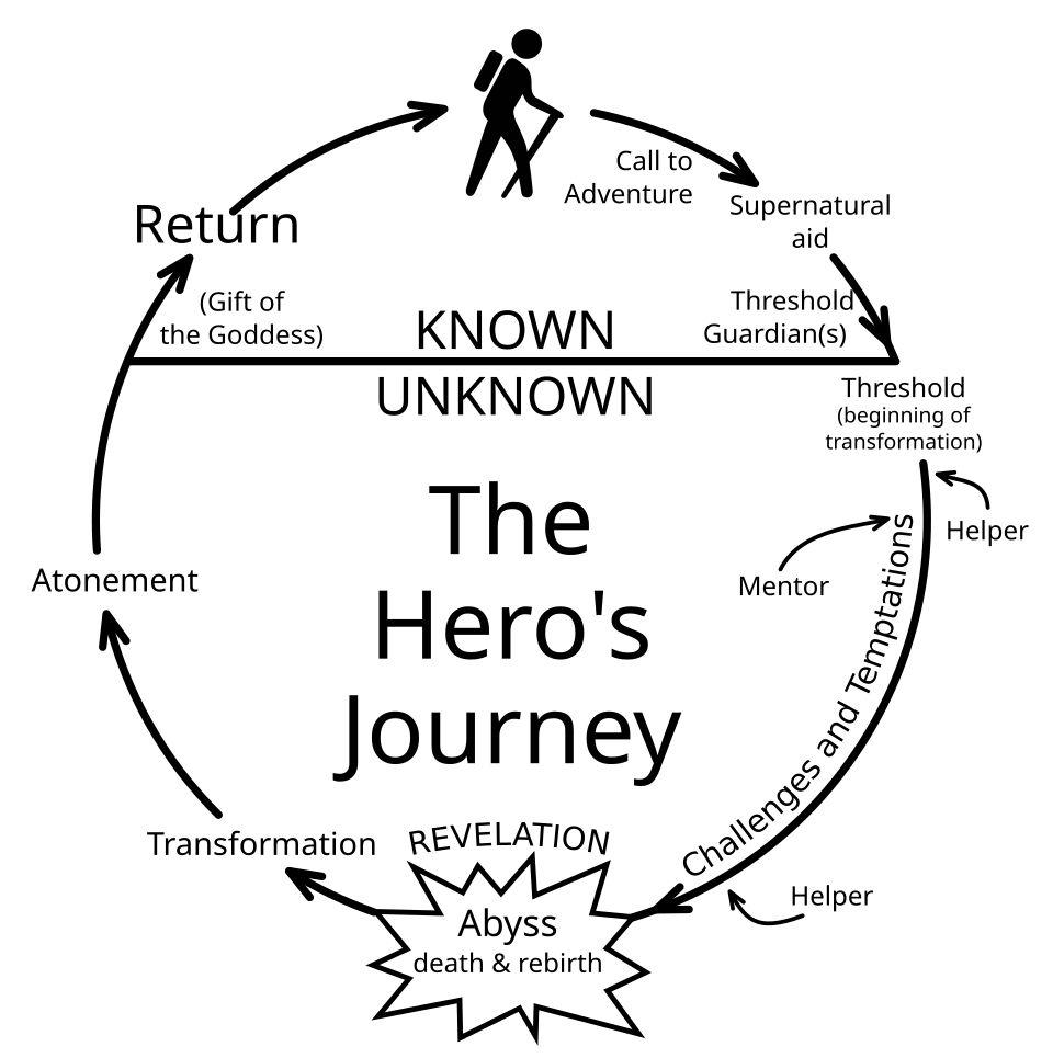
One obvious answer to this conundrum is that humans don’t remember or analyze stories in their entirety, but only consider abstractions of stories. Various theorists have tried to build models of specific stories, or classes of stories. The most well-known of these is Campbell’s “Hero’s Journey”, from The Hero with a Thousand Faces (1949).
There is an entire corpus of scholarly work attempting to build narratological models of stories.
Most of the academic work seems aimed at classifying or characterizing existing stories. These range from role-based models (Greimas models stories as interactions among a small set of roles) to grammars (Vladimir Propp’s Morphology of the Folktale, which treats Russian folktales as sequences of standardized “functions” that behave roughly like the states of a finite-state automaton).
In folklore, academics have even attempted to index the space of known plots. The Aarne–Thompson–Uther (ATU) folktale type index assigns each traditional tale a numeric “type” (ATU 510A for “Cinderella”, 300–749 for various hero tales, and so on), while Stith Thompson’s Motif-Index of Folk-Literature catalogues recurring “mythemes”, story motifs like “cruel stepmother,” “magic helper,” “journey to the underworld”. In effect, these systems treat the corpus of folktales as a finite catalogue of plot skeletons and motifs that can be recombined.
There’s also a small cottage industry of “implementable” story frameworks aimed at aspiring screenwriters (Syd Field’s three-act paradigm, Snyder’s “Save The Cat”, John Truby’s Anatomy of Story) which break all stories down into a “templated” set of steps (to be implemented by a writer)3.
Finally, there are attempts to embed stories (and indeed, all of language) into low-dimensional spaces using machine learning. These are outside the scope of this post.
Long story short: long stories can be made short.
Counting Abstract Stories
Now that we’ve concluded stories can be abstracted, let’s investigate the “crowdedness” of the space of stories. Let’s suppose a story’s “semantic type” can be encoded in only \(k\) “semantic” bits4, similar to our analysis of pictures. If there are \(N\) “evenly distributed” stories, how close are they to each other?
To be clear, we are modeling each “abstract story” in our model as a string of 1s and 0s. Each bit represents some abstract story element (for example, “comedy or tragedy”). We can view this as an “index” into the set of stories (like in Borges’ library). If a story differs from another story in \(r\) bit places, we say the two stories are “Hamming distance \(r\)” away from each other.
We can also similarly assume each story “claims” the nearby \(r\) radius. Then the “volume” of the Hamming neighborhood is:
\[ V(k, r) = \sum_{i=0}^{r} {k \choose i} \]
Therefore, we say there are \(V(k, r)\) stories within radius \(r\) of the original story.
Since there are \(2^k\) stories total, if we assume the stories are evenly distributed5, we get (crudely)
\[ N\cdot V(k,r) \approx 2^{k} \]
Suppose we want to create a new story in this space. What’s the minimal overlap it will have with an existing story?
If we know \(N\) and \(k\), we can find this by solving the following equation for \(r\):
\[ V(k, r) \approx \frac{2^{k}}{N} \]
and then computing “bits in common”
\[ d_0 = k - r \]
in fractional form:
\[ d_{f} = \frac{d_{0}}{k} = 1 - \frac{r}{k} \]
How large are \(N\) and \(k\) in reality?
Let’s stick with English. For novels, according to Fredner, \(N \approx 5\times 10^6\). Let’s use this estimate for now (although in reality the number of novels is dwarfed by the number of short stories, and to consider all stories we might also want to consider narrative poems, film scripts, etc.).
Reusing our semantic bit estimate of \(k=50\):
\[ \frac{2^{50}}{5000000} = \sum_{i=0}^{r} {50 \choose i} \]
Solving this, we get somewhere between \(r=7\) and \(r=8\). So \(d_f\) is bounded by \(1 - \frac{8}{50} = 0.84\).
That is, under this model, a new novel would semantically overlap with an existing story by 84% or more.
Let’s look at how varying \(k\) and \(N\) affect this result.
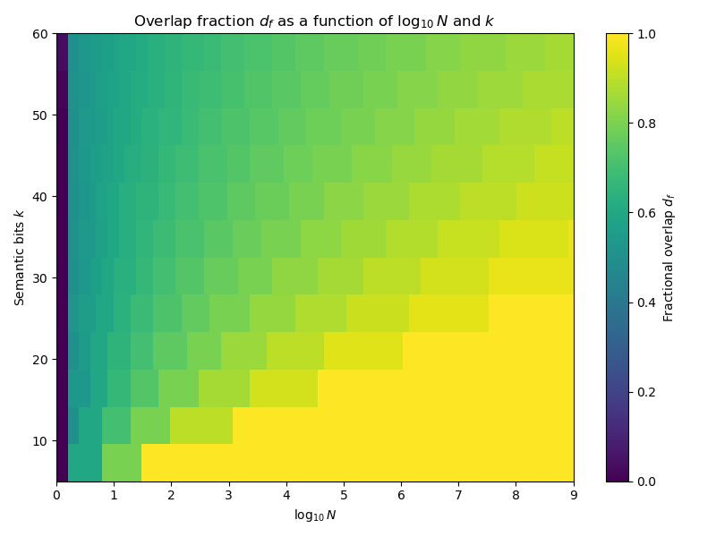
This first figure is a heatmap. We vary \(\log_{10}N\) on the x-axis and \(k\) on the y-axis. The color of the grid depends on \(d_f\).
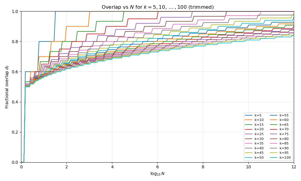
In the second plot we instead compare \(N\) to \(d_f\) for each value of \(k\).
\(d_f\) rises sharply at low \(N\), then approaches 1 as \(N\) grows larger.
So even at relatively high \(k\), the space of stories is somewhat crowded at \(10^6\). What’s more, most of the crowding occurs early, then slows down, with “steeper crowding” occurring at lower \(k\).
This matches what we expect. Stories are getting crowded. Even before we bring in energy or dynamics, a simple packing argument already suggests that most new stories must live semantically close to ones we’ve already told.
Not All Bits Are Equal
By using “semantic bits” we have implicitly assumed that the bits are (mostly) orthogonal and ordered by importance. In reality, the first bit (e.g. “tragedy vs. comedy”, or more likely some division of two common story structure types) probably matters more to human perception than the 47th bit. So our original model is a bit naive. Let’s try to improve it by adding weighting for perceptual importance.
If there is a recursive hierarchical decomposition of meaning (i.e. at the top level is comedy vs. tragedy, comedy splits into romantic comedy vs. dark comedy, etc.), and this is “scale-free”, we should wind up with a power law. Many similar natural phenomena follow power laws, such as Zipf’s Law6, which comes up in the relative frequences of words in natural corpora of texts.
So let’s assume the importance \(w_i\) of the \(i\)-th bit roughly follows a power law:
\[ w_i \propto i^{-\beta} \]
where \(\beta\) is some weight.
So we can compute the weighted distance between two works (note the shift by one to keep \(0\) indexing, consistent with the last example):
\[ d(x,y) = \sum_{i=0}^{k-1} \frac{1}{(i + 1)^{\beta}}|x_i - y_i| \]
\(x\) and \(y\) are strings in this case, and the sum is over their characters. \(|x_i - y_i|\) returns 0 if the characters are equal, and 1 if they are different.
So the complete diameter of the space (the distance between the furthest two objects, for example the string of \(k\) “1”s and the string of \(k\) “0”s) is:
\[ d(11111..1,00000..0) = \sum_{i=0}^{k-1} \frac{1}{(i + 1)^{\beta}} \]
This is the partial sum of the \(p\)-series7. In the limit, the \(p\)-series only converges for \(\beta > 1\). Call the partial sum \(S_{k}(\beta)\) for a given \(\beta\).
Now let \(R\) be the typical nearest-neighbor distance between works in this weighted metric. We’ll also assume there’s a perceptual threshold distance \(R_c\) below which differences between works become imperceptible. This threshold probably varies by person: more casual consumers have a higher \(R_c\), whereas experts have a lower \(R_c\).
For a given \(k\) and \(\beta\), \(S_k(\beta)\) is the maximum possible distance. If the typical nearest-neighbor distance \(R\) falls well below a perceptual threshold \(R_c\), then most works within that ball of radius \(R_c\) will feel indistinguishable to a given observer. When \(R\) is still a substantial fraction of \(S_k(\beta)\), there is still plenty of perceptual room for works to feel distinct.
We can now repeat our earlier analysis.
Let \(V_\beta(k,R)\) be the number of strings within weighted distance \(R\) of a given string. Then by our crude packing argument we get a volume:
\[ V_{\beta}(k, R) = \frac{2^{k}}{N} \]
and a new weighted \(d^w_f\)
\[ d^w_f = 1 - \frac{R}{S_k(\beta)} \]
Given \(S_k(\beta)\), we can solve implicitly for \(R\).
There’s three different cases for what the approximation of \(S_k(\beta)\) looks like, depending on \(\beta\).
\[ S_k(\beta) \approx \begin{cases} \dfrac{k^{1-\beta}}{1-\beta}, & 0 < \beta < 1, \\[6pt] \log k + \gamma, & \beta = 1, \\[6pt] \zeta(\beta) - \dfrac{1}{(\beta-1)\,k^{\beta-1}}, & \beta > 1, \end{cases} \]
where \(\zeta(\beta)\) is the zeta function, and \(\gamma\) is the Euler-Mascheroni constant. Note that the partial sum only actually converges in the limit if \(\beta \gt 1\).
Let’s think about each case.
Case 1: \(0 \lt \beta \lt 1\)
In this case, the partial sum diverges like a polynomial in \(k\). \(S_k({\beta}) \approx \frac{k^{1-\beta}}{1 - \beta}\)
The intuition is that the weights fall off very slowly as we progress to increasingly low-order bits, so “low-order” bits still contribute meaningfully to perception (though less than higher-order bits).
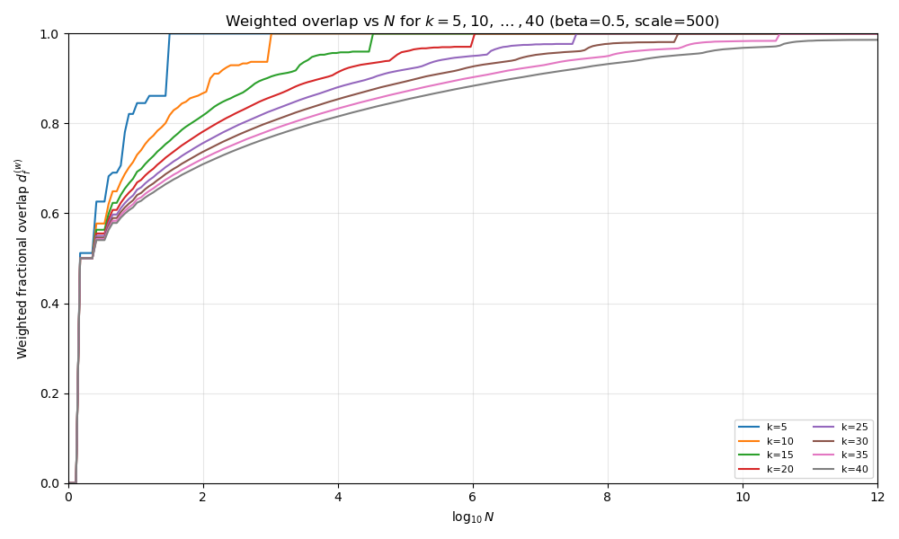
Plot above at \(\beta = 0.5\).
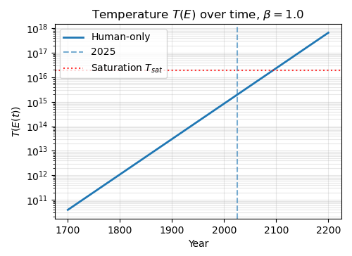
Case 2: \(\beta = 1\)
In this case, we have a harmonic series, and the partial sum is roughly a logarithm in \(k\):
\[ S_k(1) \approx \log(k) + \gamma \]
In this case, each bit is worth roughly the same. This is the “Zipfian” case.
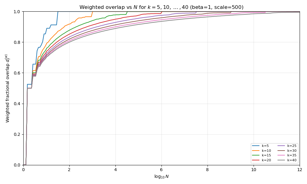
Plot above at \(\beta = 1\).
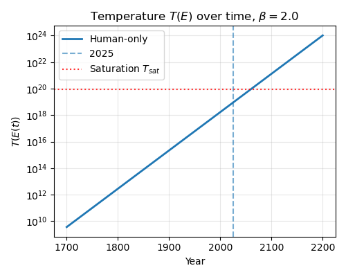
Case 3: \(\beta \gt 1\)
Finally, if \(\beta \gt 1\) we have a convergent series. The partial sum \(S_k\) converges to the zeta function \(\zeta(\beta)\) in the limit, plus an additional term (\(S_k(\beta) \approx \zeta(\beta) - \frac{1}{(\beta-1)\,k^{\beta-1}}\)).
In this regime, marginal bits are worth much less than earlier bits: most of the perceptual “distance budget” is carried by the first few coordinates. Geometrically, the metric has a finite diameter (bounded by \(\zeta(\beta)\)) even as the number of distinct works \(2^k\) grows exponentially. Beyond some point, adding more bits creates many more states that are all crammed into almost the same finite perceptual space.
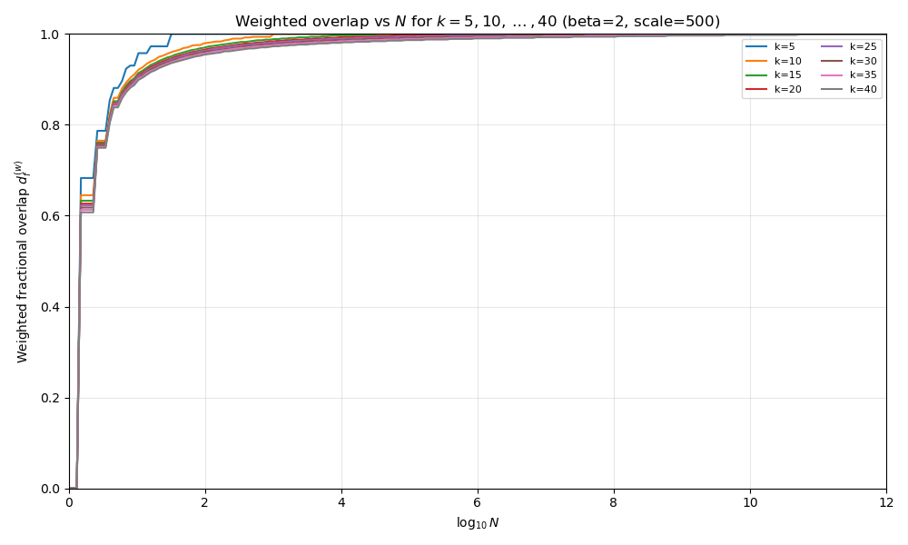
Plot above at \(\beta = 2\). See how it is noticeably more “squashed” than the last two?
Dynamics
Now that we have a method to measure the “crowdedness” of the space is terms of the total number of possible artifacts, let’s look at production in terms of total spent energy, and how that relates to the amount of novelty remaining. If we can link energy spent to the number of remaining microstates, we can use methods from statistical mechanics to model the state of the culture, and how it will change over time.
Empirical Energy Estimates
Let’s do some Fermi estimates of the total energy expenditure spent over time to reach the current cultural stock.
Let’s break this down.
\[ N_{\text{novels}}\cdot\frac{\text{time}}{\text{novel}} \cdot \frac{\text{energy}}{\text{time}} = \text{energy} \]
We already estimated \(5\times 10^{6}\) total novels. If a novel takes roughly 800 hours8, and a human burns 135 watts while writing9, we get:
\[ 5\times 10^6 \cdot 800 \cdot 60 \cdot 60 \cdot 135 \approx 10^{15} \text{J} \]
or \(10^{15}\) total joules (roughly 10 Hiroshima-class atomic bombs).
That’s the metabolic energy to actually produce the works. We’ll pretend that all works are magically placed in the library instantly, but note that there is also some additional analysis possible regarding distribution10.
Statistical Mechanics of Semantic Space
Can we now connect the energy input to our model of cultural generation?
Let’s arbitrarily choose a reference frame, the \(k\)-length string \(0\) = “000..0”11.
We can then compute the “internal energy” \[ E^\ast(x) = d(x, 0) = \sum_{i=0}^{k-1} \frac{x_i}{(i + 1)^{\beta}} \]
The number of microstates \(\Omega(E)\) for a given energy level \(E\) is:
\[ \Omega(E)=\#\{x\in\{0,1\}^k : E^\ast(x)\le E\} \]
That is, for a given \(E\) and \(x\), we count up the strings where \(d(x, 0) \lt E\). We can define the “entropy” now:
\[ S = \log \Omega(E) \]
where \(\Omega\) is the number of microstates within distance \(E\) of the reference.
We are actually seeking the “novelty” per unit energy added to the system. This looks like
\[ \frac{\partial S}{\partial E} \]
It just so happens that this is related to the temperature.
\[ \frac{1}{T} = \frac{\partial S}{\partial E} \]
which we can approximate as
\[ \frac{1}{T} = \frac{\partial S}{\partial E} \approx \frac{\Delta S}{\Delta E} = \frac{\log(\Omega(E + (k + 1)^{-\beta})) - \log(\Omega(E))}{(k + 1)^{-\beta}} \]
Solving for \(T\)
\[ T \approx \frac{(k + 1)^{-\beta}}{\log(\Omega(E + (k + 1)^{-\beta})) - \log(\Omega(E))} \]
So (by definition) as \(T\) increase, the marginal entropy (the amount of space for new stories) per unit of marginal energy declines.
Using the \(k=50\) and \(N=5\times 10^6\), we can plot \(T\) against the total cumulative energy added to the system \(\mathcal{E}\):
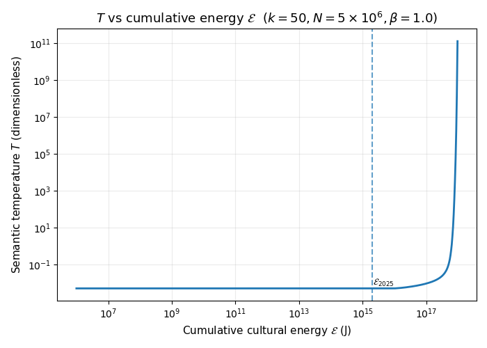
The above plot is at \(\beta=1.0\). Basically, the temperature doesn’t change much at first, but past a certain amount of energy \(\frac{dS}{dE^\ast}\) drops rapidly as we “run out of room” and temperature increases rapidly.
Heat Capacity
Let’s now look at the marginal gain compression (changes in \(T\)) as energy increases.
Under the microcanonical ensemble, we can define the heat capacity as
\[ C(E) = \left( \frac{\partial T}{\partial E} \right)^{-1} \]
which we can approximate as
\[ C(E) \approx \frac{\Delta E}{T(E+\Delta E) - T(E)} \]
Alternately this can be written in terms of \(S\):
\[ C(E) \approx -\,\frac{T(E)^2}{\dfrac{S(E+\Delta E) - 2S(E) + S(E-\Delta E)}{(\Delta E)^2}} \]
With the heat capacity, we can now connect the effect of the marginal energy input into the system with the change in the remaining capacity.
Intuitively, \(C(E)\) measures how the energy we pump into the system relates to increases in the effective temperature \(T\) (scarcity of novelty per unit energy).
When \(C(E)\) is large, adding energy changes \(T\) slowly. This corresponds to a regime where there is still a lot of unexplored semantic volume, and we can keep investing in new works without running out of “cheap” novelty.
When \(C(E)\) is small, adding a little energy produces a big jump in \(T\). In this regime, most of the low-hanging novelty has already been harvested, so further investment mostly churns inside already-occupied regions of semantic space.
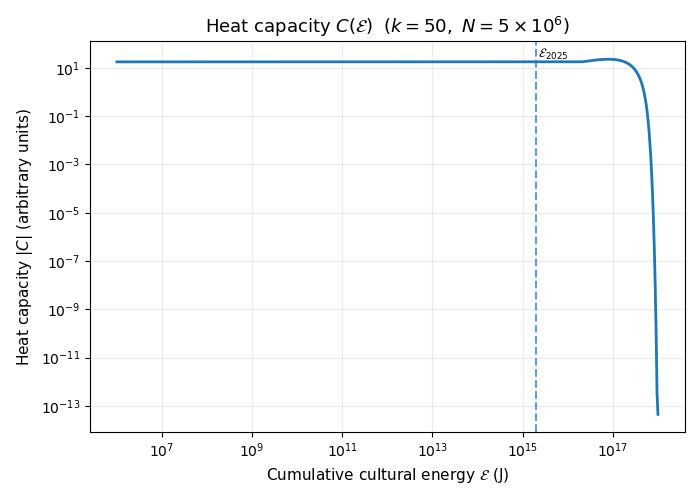
If we plot the heat capacity against total energy added to the system, we see the heat capacity is pretty constant until it suddenly declines.
Synthesis
Let’s put the argument together and examine the dynamics of this situation from a society-level perspective. Human society expends energy (in the form of food and fuel) to find cultural objects. How much energy does it take to find “novel” cultural objects?
We can connect the entropy change over time to the energy input \(\dot E\) and the temperature \(T\):
\[ \frac{dS}{dt} = \frac{\partial S}{\partial E}\,\frac{dE}{dt} = \frac{\dot E(t)}{T(E)} \]
For now, let’s assume a constant energy input rate. Therefore
\[ \dot E(t) = \kappa \]
and so
\[ E(t) = E_0 + \kappa t \]
Let’s recall our three cases and go case-by-case
Case 1: \(0 \lt \beta \lt 1\)
This is our “slow drop off” case. In the \(0 < \beta < 1\) regime, the earlier bit-weight analysis gave a polynomial growth of the effective “diameter” with \(k\),
\[ S_k(\beta) \approx \frac{k^{1-\beta}}{1-\beta} \]
and if we take energy to be proportional to \(k\) we can write entropy \(S\) as a power law in \(E\):
\[ S(E) \approx A E^{1-\beta} + B \]
for some constants \(A > 0\), \(B\).
Then
\[ \frac{dS}{dE} = A (1-\beta) E^{-\beta} \]
Using \[ \frac{1}{T(E)} = \frac{dS}{dE} \]
we obtain
\[ \frac{1}{T(E)} = A (1-\beta) E^{-\beta} \] \[ T(E) = \frac{1}{A(1-\beta)}\,E^{\beta} \]
The entropy production rate under constant energy input is
\[ \frac{dS}{dt} = \frac{dS}{dE}\,\dot E = A (1-\beta) E^{-\beta} \kappa = \frac{A (1-\beta) \kappa}{\bigl (E_0 + \kappa t\bigr)^{\beta}} \]
So, given constant energy input \(\frac{dS}{dt}\) falls off as \(O(t^{-\beta})\). Alternatively, each doubling of our energy input should yield \(2^{-\beta}\) amount of “novelty”.
Case 2: \(\beta = 1\)
This is our Zipfian case. Before, we had
\[ S_k(1) \approx \log k + \gamma \]
so suppose
\[ S(E) \approx a \log E + b \]
with \(a\) and \(b\) constants. Then
\[ \frac{dS}{dE} = \frac{d}{dE}\bigl(a \log E + b\bigr) = \frac{a}{E} \]
Using \[ \frac{1}{T(E)} = \frac{dS}{dE} \]
we get
\[ \frac{1}{T(E)} = \frac{a}{E} \]
\[ T(E) = \frac{E}{a} \]
With constant energy input, \[ E(t) = E_0 + \kappa t \]
therefore
\[ \frac{dS}{dt} = \frac{dS}{dE}\,\dot E = \frac{a}{E(t)}\,\kappa = \frac{a\kappa}{E_0 + \kappa t} \]
Integrating in time:
\[ S(t) \approx a \log\bigl(E_0 + \kappa t\bigr) + b \]
So in the Zipfian regime, even with constant energy input, entropy (the number of distinguishable cultural microstates) grows logarithmically in time. Equivalently, exponential energy input leads to linear growth output.
Sound familiar? This is similar to the story we heard earlier, related to science.
Case 3: \(\beta > 1\)
This is the bounded regime. Since the p-series converges to a finite limit for \(\beta > 1\), there is an effective maximal energy scale \(E_{\max}\) and corresponding maximal entropy
\[ S_{\max} = \log \Omega(E_{\max}) \]
We can’t do the same analysis we did in the previous two cases because the number of bits is no longer proportional to the energy. That being said, we can reason intuitively that under constant energy input, \(T(E)\) diverges as \(E \to E_{\max}\), while the entropy production rate \(\dfrac{dS}{dt}\) collapses to zero.
Time to Saturation
How far are we from saturation? More specifically, given some energy input rate \(\dot E = \kappa\), how long does it take before novelty per unit time falls below the perceptual threshold \(R_c\), or before we’ve exhausted a fixed fraction of the available semantic space?
We can find this by computing:
\[ t_{\text{sat}} = \frac{E_{\text{sat}} - E_0}{\kappa} \]
We have expressions for \(E\) from the previous section, and we have estimates for \(E_0\) and \(\kappa\). To find \(E_{\text{sat}}\), we compute \(V(k, R_c)\), then compute \(E_{\text{sat}} = \frac{2^k}{V(k, R_c)E_{\text{work}}}\).
I’ll omit the details. We can now plot out the dynamics using software.
Plots
AI Disclosure: Don’t take these plots too seriously. They’re mostly for illustrative effect. The parameter choices and saturation threshold are arbitrary; the only thing that really matters is the qualitative shape: initially flat, then a sharp rise once the space becomes crowded.
Now that we know how to compute everything, let’s take a look at historical and future trends. Instead of a universally constant energy input rate, let’s assume roughly exponential increase in energy input starting at the year 1700. There were also very few English language novels in the year 1700, so I used “100” as an approximation.
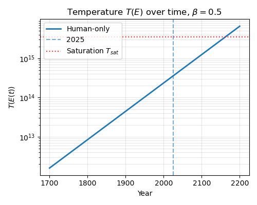
These are toy graphs. The saturation level is arbitrary. In the above graphs I’ve just set it to 10x the current temperature. But we can see that the saturation point could be quite close, especially if we think \(\beta\) is high.
Regardless, under these assumptions, the qualitative picture is straightforward. At first, additional energy buys a lot of entropy. The system is “cold”, and new works carve out genuinely new regions of semantic space. As cumulative energy grows, the effective temperature \(T(E)\) remains roughly flat for a while, then begins to rise rapidly as we enter the crowded regime. Beyond that point, most of the marginal energy goes into producing works that sit inside already-populated neighborhoods in story space, rather than opening up genuinely new directions.
Now, let’s imagine that AI lets us move past metabolic limits for cultural production sometime in the near future. What will that do to our saturation times? The computations are easy: time to saturation and energy required are proportional in this framework. For example, AI might let us instantly increase the energy rate used to mine culture by one or more orders of magnitude. How does the projection change?
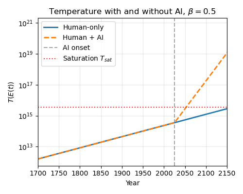
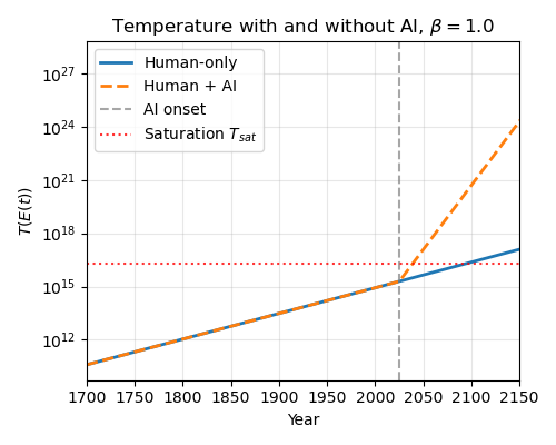
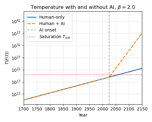
Here I’ve let AI increase energy expenditures by 5x. This massively decreases the saturation timeline
Negative Temperature
The \(\beta > 1\) case (especially high \(\beta\)) has some especially interesting properties. In this case we can get “negative temperature”.
In ordinary thermodynamic systems, adding energy increases the number of accessible microstates, so \(S(E)\) is increasing and \(\frac{\partial S}{\partial E} > 0\), which implies a positive temperature. In some long-range interacting systems, however, the density of states is not monotonic. Beyond a threshold, adding more energy actually reduces the number of accessible microstates, so \(\frac{\partial S}{\partial E} < 0\) and the effective temperature becomes negative.
Onsager’s classic example is a gas of point vortices in two dimensions. At low energy you get many small, disordered vortices but at very high energy the system prefers to concentrate that vorticity into a few large, coherent “supervortices.” These macroscopic structures are more “ordered,” but they correspond to the highest energies and thus to negative temperature states.
If we push the cultural analogy, a negative-temperature regime in semantic space would be one where driving the system to higher “energy” (more extreme, differentiated works) eventually reduces the number of distinct configurations, because the only way to pack that much structure into a bounded perceptual manifold is to form large-scale superstructures.
Maybe this is already happening? Mega-franchises, shared universes… all are examples of canonical templates that organize huge numbers of micro-variations. In such a regime, additional energy no longer produces fine-grained diversity. Instead, adding energy reinforces a few giant, highly ordered attractors that dominate the landscape.
Conclusion
We’ve built a simple model of the space of stories using methods inspired by statistical mechanics. The model shows that, over time, the space of stories becomes more crowded. If we increase the amount of energy we pour into constructing cultural objects, the space will “run out” more quickly. As we proceed, innovation happens in “lower-order” bits.
How seriously should we take this? Since there’s such a huge amount of stories, it seems outlandish that we could actually run out. Regardless, I think this exercise is useful as a first step in tying some of the intuition I’m developing around information bottlenecks to physical and social processes.
Additional Thoughts
In no particular order:
It’s possible that \(\beta\) differs based on different segments of the population.
If there are different segments of the population at different \(\beta\), do they proceed independently through this progression? Will “intellectual superfranchises” emerge?
\(\beta\) could vary along the “bit direction”. So early bits are at a different \(\beta\) than later bits.
Since human intelligence is bounded, the space of stories must ultimately be bounded.
Stories are not actually evenly distributed. However, this doesn’t necessarily weaken the argument. In fact, if there are a limited number of “story attractors”, then we would expect some regions of story space to actually grow more crowded more quickly.
There may be additional modeling that could be done here. For example, can this model predict punctuated equilibrium? Maybe there are regions that are separated by “high-energy barriers” or areas of extremely low density. Maybe the semantic manifold has disconnected or quasi-disconnected components.
If something like Propp’s model could be made into a full-out recursive structure (like a context-free grammar), does this change the analysis? Then we are not necessarily looking at “fixed strings”.
Stories can be forgotten, freeing up space for stories to reoccur.
Are there empirical ways to test this model? What concrete, falsifiable hypotheses does it make?
AI Disclosure
Probably the most heavily I’ve used AI on a post. I used ChatGPT and Claude to make a bunch of the graphs (an extremely painful process, I ended up making several graphs myself), to format LaTeX, to find sources, and for general feedback and brainstorming.
Footnotes
A grammatical English text of length \(L\approx 8\times 10^4\) words has about \(C \approx 6L\) characters. Using an entropy rate of \(h\approx 1\)–\(1.5\) bits/char (a conservative estimate) gives total information \(B \approx hC \approx 1 \text{ to } 1.5 \frac{\text{bits}}{\text{char}}\times 6 \frac{\text{chars}}{\text{word}} \times L \text{ words} \approx (5\times 10^5 \text{ to } 7.5\times 10^5)\ \text{bits}.\) Thus the number of grammatical English sequences is \(N \approx 2^B \approx 10^{0.301B} \sim 10^{(1.4\times 10^5 \text{ to } 2.2\times 10^5)}.\) If we assume the “empty word” is in our vocabulary, we can include shorter works in the same counting argument.↩︎
See here, here or here for some claims about science. While this essay focuses on culture, it’s possible similar arguments apply to other intellectual pursuits. We may even see some similar input-output relationships. That being said, science, math, and code have inductive structures that render some of this analysis less pertinent. For example, in math, a theorem might be stated very simply but imply an extensive proof of unknown length. Perhaps more on this in a future post.↩︎
It would be interesting to see attempts to combine these resources with LLMs to construct new stories.↩︎
We will get into the value of \(k\) later.↩︎
We will examine this assumption later.↩︎
Claude suggested that, under a Chinese Restaurant Process or stick-breaking construction, the resulting ranked piece sizes follow a \(w_i \propto \frac{1}{i}\) distribution due to a connection between Dirichlet processes and Zipf’s law. This is also potentially related to pink noise.↩︎
https://math.stackexchange.com/questions/2848784/general-p-series-rule↩︎
https://www.jenniferellis.ca/blog/2016/8/27/hourstowriteanovel. Seems reasonable AFAICT.↩︎
I assume 35% over a baseline 100 watt human.↩︎
This is a bit weird because you could have cases where some consumers have access to some works but not others. It seems outside the scope of this post.↩︎
A better reference frame would probably be somehow drawn from the typical set, and then the “higher-energy” texts would be more ordered, but I couldn’t figure out how to do this properly. Possibly the metric should be engineered along these lines as well.↩︎