Controls from the Geometric Perspective

Introduction

In my post on differential games and stag hunt I mentioned discrete controls. When looking into this topic, I ended up in a rabbit hole around geometric controls. To learn a bit more, I took a look at the paper Discrete Control Systems, by Taeyoung Lee, Melvin Leok, N. Harris McClamroch, but many parts of the exposition diverged from the paper as I proceeded in my investigation.

In particular, I wanted the control problem to motivate the Lagrangian, rather than deriving the Lagrangian in terms of the desired physics.

AI Disclosure: I used ChatGPT to generate a bunch of the LaTeX in this post. Mistakes my own.

Background

Consider some system with configuration space \(Q\).

\(Q\) is a set, and each element \(q\) of \(Q\) is one particular configuration. For mechanical systems, \(Q\) would be all possible positions of the system and \(q\) would be a particular position. \(Q\) might be a particle location in 3D (\(Q = \mathbb{R}^3\)), the orientation of a rigid body (\(Q = SO(3)\)), or something else.

Suppose the system starts in configuration \(q_0\) and we want it to be in \(q_N\). Which path should we take to transform the configuration? We can frame this problem using the Lagrangian. However, first we need to assume a bit more about \(Q\), namely that it is smooth manifold equipped with a Riemannian metric and a tangent bundle¹.

Manifold

\(Q\) is a smooth manifold of dimension \(n\) if around every point \(q \in Q\) we can find a neighborhood \(U\) and a map \(\phi\) such that

\[ \phi : U \to \mathbb{R}^n \]

that is bijective, infinitely-differentiable, and has a smooth inverse \(\phi^{-1}: \mathbb{R}^n \to U\). We call the map \(\phi\) a chart, or coordinate system.

Furthermore, we require overlapping charts to agree smoothly. In practical terms, this means we have two differentiable functions:

def to_local_coords(self, q, center):
    raise NotImplementedError
    
def from_local_coords(self, x, center):
    raise NotImplementedError

such that from_local_coords(to_local_coords(q, center), center) = q (at least approximately) and vice-versa.

For a Euclidean space (\(Q = \mathbb{R}^3\)), \(\phi\) is simply the identity.

Riemannian Metric

To get a Riemannian manifold, there is a second requirement. At each point \(q \in Q\), we construct the tangent space \(T_qQ\) of all possible velocity vectors at \(q\) (keep in mind we said \(Q\) was infinitely differentiable). We also have an inner product \(g_q\) at each point \(q\)

\[ g_q : T_qQ \times T_qQ \to \mathbb{R} \]

To be a Riemannian metric², \(g_q\) needs to meet the following four conditions:

1. \(g_q(v_1, v_2) = g_q(v_2, v_1)\) (Symmetry)
2. \(g_q(av_1 + bv_2, w) = ag_q(v_1,w) + bg_q(v_2, w)\) and \(g_q(v, aw_1 + bw_2) = ag_q(v,w_1) + bg_q(v, w_2)\) (Bilinearity)
3. \(g_q(v,v) > 0\) for all \(v \neq 0\) (Positive Definite)
4. For every chart \(\varphi: U \to \mathbb{R}^n\), the metric components \(g_{ij}(x) = g(\partial_i, \partial_j)\) in coordinates are \(C^\infty\) (Smooth)

Basically, to implement our (now Riemannian) manifold, we will need something like:

class Manifold:
    """Base class for smooth manifolds"""
    
    def metric(self, q, v1, v2):
        raise NotImplementedError
    
    def inner_product(self, q, v1, v2):
        return self.metric(q, v1, v2)

Tangent Bundle

The tangent bundle \(TQ\) is defined as the collection of all position and velocity pairs:

\[ TQ := \{(q, v) : q \in Q, v \in T_qQ \} \]

Lagrangian

Now that we have established the structure, we can define the Lagrangian.

The Lagrangian is a (smooth) function that assigns a number to each element of the tangent bundle:

\[ L : TQ \to \mathbb{R} \]

The Lagrangian encodes a “cost” for each way of moving through the configuration space. Given any trajectory \(q(t)\) from \(q_0\) to \(q_N\), we can evaluate its goodness by computing the action:

\[ S[q] = \int_{t_0}^{t_N} L(q(t), \dot{q}(t)) \, dt \]

The action \(S\) assigns a single number to each possible path. Hamilton’s Principle states that the physically realized path the one where nearby paths have approximately the same action (that path is a critical point in the space of paths).

Euler-Lagrange Equations

Consider a trajectory \(q(t)\) and a small variation in that trajectory \(\eta(t)\) with fixed endpoints. We know that \(\eta(t_0) = \eta(t_N) = 0\), because the system must still start and end at the desired configurations (we have just varied the path). Thus the varied path is:

\[ q(t) + \epsilon\eta(t) \]

for small \(\epsilon\). The action along the varied path is

\[ S(\epsilon) = \int_{t_0}^{t_N} L(q + \epsilon \eta, \dot{q} + \epsilon \dot{\eta}) dt \]

We want our trajectory to be a critical point in the space of paths. So

\[ \frac{\partial S}{\partial\epsilon}\biggr\vert_{\epsilon = 0} = 0 \]

by differentiating under the integrand and using the chain rule, we have

\[ \frac{\partial S}{\partial\epsilon}\biggr\vert_{\epsilon = 0} = \int_{t_0}^{t_N} \big[ \frac{\partial L}{\partial q}\eta + \frac{\partial L}{\partial \dot{q}}\dot{\eta} \big] dt \]

We can break this up and integrate the second term by parts:

\[ \int_{t_0}^{t_N} \frac{\partial L}{\partial \dot{q}} \dot{\eta}\, dt = \left. \frac{\partial L}{\partial \dot{q}} \eta \right|_{t_0}^{t_N} - \int_{t_0}^{t_N} \frac{d}{dt} \left( \frac{\partial L}{\partial \dot{q}} \right) \eta\, dt \]

since \(\eta(t_0) = \eta(t_N) = 0\), the first term is zero. Substituting back we have

\[ \left. \frac{dS}{d\varepsilon} \right|_{\varepsilon=0} = \int_{t_0}^{t_N} \left[ \frac{\partial L}{\partial q} - \frac{d}{dt}\left( \frac{\partial L}{\partial \dot{q}} \right) \right] \eta\, dt = 0 \]

Since this is true for any \(\eta(t)\), the integrand is zero everywhere:

\[ \boxed{ \frac{d}{dt} \left( \frac{\partial L}{\partial \dot{q}} \right) - \frac{\partial L}{\partial q} = 0 } \]

The boxed term is the Euler-Lagrange equations.

Hamiltonian

The action functional (when we integrate over the Lagrangian) is a global principle. It cares about the entire path we have looked at. The Lagrangian itself is the infinitesimal contribution to this global quantity: it evaluates how “expensive” it is to move through a infinitesimal segment of the path.

How does that translate into an actual policy? That is, given the current state, which infinitesimal step should we take next?

The Lagrangian is a function

\[ L : TQ \to \mathbb{R} \]

\(L\) restricts locally to:

\[ L_q: T_qQ \to \mathbb{R} \] \[ v \mapsto L(q, v) \]

This is a “marginal cost” of moving from \(q\) with velocity \(v\).

Given a \(q\), how does \(L(q,v)\) change if we alter \(v\) within the tangent space \(T_qQ\)? That is, if what is the effect of a small change in speed on the marginal cost?

We perturb \(v\) in the direction \(w \in T_qQ\), the derivative in that direction at a given \(q\) and \(w\) is:

\[ p(w) := \frac{d}{d\epsilon} [L(q, v + \epsilon w)]\biggr|_{\epsilon=0} \]

We may also denote this as

\[ p := d_vL_q \]

Each \(p\) tells you how sensitive the cost is to change in \(v\).

Consider the canonical evaluation map

\[ \text{ev}_q: T^*_qQ \times T_qQ \to \mathbb{R} \] such that \[ \text{ev}_q(p, v) \mapsto p(v) \]

\(p(v)\) is the first-order predicted cost change for a given \(v\), which has the same units as \(L(q, v)\). So if we fix \(q\), we can say that for any \(v\)

\[ p(v) - L(q,v) \]

is the instantaneous “error in cost” (best affine approximation) between the linearization of \(L(q,v)\) in local coordinates (\(p(v)\)) and the “actual” instantaneous cost \(L(q,v)\).

The most consistent local description of \(L\) given \(p\) is the maximum possible value of this difference over all directions \(v\). In other words, given my sensitivity \(p\) to \(v\), and the cost \(L(q,v)\) of moving at \(v\), which \(v\) should I move at to obtain to best approximate the true global optimum? In equations, define:

\[ H(q,p) := \sup_{v\in T_qQ} (p(v) - L(q,v)) \]

This is the “fiberwise Legendre transform”. The resulting function \(H: T^*Q \to \mathbb{R}\) is called the “Hamiltonian”.

Hamilton’s Equations

To move between the “velocity picture” \((q,v)\) and the “covector picture” \((q,p)\), we need to ensure that every velocity has a unique covector representing its local rate of change of cost, and vice versa.

We already have the “fiber derivative” from before: \[ p := d_vL_q \in T_q^*Q. \]

This defines the Legendre map \[ \mathbb{F}L: TQ \to T^*Q,\qquad (q,v)\mapsto (q,p=d_vL_q). \]

For the Hamiltonian to exist as a function (rather than a possibly multivalue-relation³), \(\mathbb{F}L\) must be locally invertible. Lucky for us, the Riemannian metric \(g_q: T_qQ\times T_qQ \to \mathbb{R}\) gives us a canonical way to manage this.

Under the metric isomorphism \(g_q: T_qQ \to T_q^*Q\)⁴, we identify \[ p = g_q(v,\cdot). \]

Because \(g_q\) is positive definite and nondegenerate, this map is automatically invertible.

If we assume a unique supremum at \(v(q,p)\), and take our identity:

\[ H(q,p) = p(v(q,p)) - L(q,v(q,p)) \]

and differentiate \(H\), it gives \[ \begin{aligned} dH &= d\big(p(v(q,p))\big) - d\big(L(q,v(q,p))\big) \\[6pt] &= \big(v\,dp + p(dv)\big) - \Big( \frac{\partial L}{\partial q}\,dq + \frac{\partial L}{\partial v}\,dv \Big) \\[6pt] &= v\,dp - \frac{\partial L}{\partial q}\,dq + \big(p - \frac{\partial L}{\partial v}\big)\,dv \\[6pt] &= v\,dp - \frac{\partial L}{\partial q}\,dq. \end{aligned} \]

hence, matching on the multivariable chain rule: \[ \frac{\partial H}{\partial p}(q,p) = v, \qquad \frac{\partial H}{\partial q}(q,p) = -\,\frac{\partial L}{\partial q}(q,v). \]

Thus the evolution of \((q,p)\) is governed by the first-order flow \[ \boxed{ \dot{q} = \frac{\partial H}{\partial p}(q,p), \qquad \dot{p} = -\,\frac{\partial H}{\partial q}(q,p). } \]

These are Hamilton’s equations.

Mechanics on Lie Groups

We should also discuss Lie Groups and Lie Algebras. These become necessary when we are controlling a robot through states more complex than paths (for example, you may want to control the robots rotational orientation in space).

Lie Groups

A Lie group is a group that is also a real smooth manifold. To define one, we need a two group operations (multiplication and inversion) that are both smooth maps. That is

\[ \mu : G \times G \to G \] \[ \mu(x,y) = xy \]

is smooth.

As an standard example, consider

\[ \text{SO}(2, \mathbb{R}) = \left\{ \begin{pmatrix} \cos\varphi & -\sin\varphi \\ \sin\varphi & \cos\varphi \end{pmatrix} : \varphi \in \mathbb{R} / 2\pi\mathbb{Z} \right\}. \]

The group operation is matrix multiplication, the identity is the identity matrix, and given an element \(R\) of the Lie Group, the inverse is \(R(-\varphi)\) \[ \quad R(\varphi)^{-1} = R(-\varphi) = \begin{pmatrix} \cos\varphi & \sin\varphi \\ -\sin\varphi & \cos\varphi \end{pmatrix}. \]

Let’s say we want to track or control a rotating rigid body. We could use the Euler-Lagrange equations

\[ \frac{d}{dt} \left( \frac{\partial L}{\partial \dot{q}} \right) - \frac{\partial L}{\partial q} = 0 \]

but what is \(\frac{\partial L}{\partial \dot{q}}\) in this case? \(R\) is a rotation matrix satisfying \(R^TR = I\) and \(\text{det}(R) = 1\). The derivative \(\dot{R}\) must preserve this structure, and we can’t just add or subtract rotation matrices.

For any time-dependent configuration \(g(t)\) in a Lie group, we always have \[ g(t)^{-1} g(t) = \mathrm{id}_G. \]

Differentiating,

\[ \frac{d}{dt}[g^{-1}(t)]\, g(t) \;+\; g^{-1}(t)\, \dot g(t) \;=\; 0. \]

Rearranging,

\[ g^{-1}(t)\,\dot g(t) = -\,\frac{d}{dt}[g^{-1}(t)]\, g(t). \]

We define

\[ \omega(t) := g^{-1}(t)\,\dot g(t), \]

so that

\[ \dot g(t) = g(t)\,\omega(t). \]

So \(\omega(t)\) is the unique object such that multiplying it by \(g(t)\) reconstructs the time-derivative of the motion. Therefore, \(g^{-1}\dot{g} = \omega\).

Consider now the path: \(\gamma(s) := g^{-1}(t)g(t+s)\):

At \(s = 0\), we have \(\gamma(0) = \text{id}_G\). For any other \(s\), we have that \([\dot{\gamma}(s)]\biggr|_{s=0} = g^{-1}\dot{g} = \omega\). So any \(\omega\) is a derivative of a path at the identity.”

Hence, \(\omega \in T_eG\), the tangent space at the identity of the Lie Group.

Lie Algebras

The tangent space at the identity of a Lie Group \(G\) is called the Lie Algebra (Lie Algebras are denoted in mathfrak).

\[ \mathfrak{g} = T_{e}G \]

It has some nice properties:

1. It’s a vector space (can add velocities, scale them).
2. All velocities in the group can be written as \(\dot{g} = g\omega\) for some \(\omega \in T_eG\).

As we determined in the last section, we know that \(\dot{g} = g\omega\), where \(\omega = g^{-1}\dot{g} \in \mathfrak{g}\). Since the \(\omega\) live inside a vector space, if we could rewrite the Euler-Lagrange equations in terms of \(\omega\), we could use the vector space structure to add and scale them! This would solve our problem.

Euler-Poincare’ Equation

So, we want to rewrite the Euler-Lagrange equations in terms of \(\omega\).

We know \[ \omega = g^{-1}\dot{g} \]

The Lagrangian is thus \[ L(g, \dot{g}) = L(g*\text{id}_G, g*\omega) \]

If we assume the Lagrangian is left-invariant⁵, then we have

\[ L(\text{id}_G, \omega) \]

Call this the “reduced lagrangian”

\[ \ell: \mathfrak{g} \to \mathbb{R} \]

\[ \ell(\omega) := L(\text{id}_G, \omega) \]

Let’s now think of the curves

\[ \omega(t) = g(t)^{-1}\dot{g}(t) \]

We will use the same trick we did to derive Euler-Lagrange, where we modify the path by \(\epsilon\) and then find a critical point with respect to the variation.

Define the variation:

\[ \delta g(t) := \frac{\partial g_{\epsilon}(t)}{\partial \epsilon}\biggr{|}_{\epsilon=0} \]

The endpoints are fixed, and hence have variation \(0\).

So we have

\[ \eta(t):= g(t)^{-1}\delta g(t) \in \mathfrak{g} \]

or

\[ \delta g(t) = g(t)\eta(t) \]

Now define, for each \(\epsilon\), \[ \omega_\varepsilon(t) := g_\varepsilon(t)^{-1} \frac{\partial g_\varepsilon(t)}{\partial t} \]

We want: \[ \delta \omega(t) := \left.\frac{\partial \omega_\epsilon(t)}{\partial \epsilon}\right|_{\epsilon=0} \] in terms of \(\omega\) and \(\eta\).

Start with \[ \omega_\epsilon = g_\epsilon^{-1}\dot{g}_\epsilon \]

Differentiate with respect to \(\epsilon\)⁶: \[ \delta \omega = (\delta g^{-1}) \dot{g} + g^{-1} \delta \dot{g} \]

Compute \(\delta g^{-1}\) using the identity \(g_\epsilon g_\epsilon^{-1} = \text{id}_G\): \[ \delta g^{-1} = -\,g^{-1} (\delta g)\, g^{-1} \]

Compute \(\delta \dot{g}\): \[ \delta \dot{g} = \frac{\partial}{\partial t}(\delta g) = \frac{\partial}{\partial t}(g\eta) = \dot{g}\,\eta + g\dot{\eta} \]

Substitute both into the expression for \(\delta\omega\):

\[ \begin{aligned} \delta \omega &= (\delta g^{-1})\dot{g} + g^{-1}\delta\dot{g} \\[4pt] &= \big(-g^{-1}(\delta g)g^{-1}\big)\dot{g} + g^{-1}(\dot{g}\,\eta + g\,\dot{\eta}). \end{aligned} \]

Now insert \(\delta g = g\eta\) and simplify:

\[ \begin{aligned} -g^{-1}(g\eta)g^{-1}\dot{g} &= -\eta (g^{-1}\dot{g}) = -\eta\omega\\ g^{-1}\dot{g}\,\eta &= \omega\eta\\ g^{-1}g\,\dot{\eta} &= \dot{\eta} \end{aligned} \]

So we have \[ \delta \omega = \dot{\eta} + \biggr( \omega\eta - \eta\omega \biggr) \]

The second term is called the “Lie bracket” and denoted:

\[ [\omega,\eta] := \omega\eta - \eta\omega \]

So: \[ \boxed{\delta \omega = \dot{\eta} + [\omega, \eta]} \]

The action over the reduced Lagrangian is \[ S[\omega] = \int_{t_0}^{t_1} \ell(\omega(t))dt \]

Vary it:

\[ \delta S = \int_{t_0}^{t_1} \frac{d}{d\epsilon} \biggr[\ell(\omega + \epsilon \, \delta \omega)\biggr]_{\epsilon=0} dt \]

\[ = \int_{t_0}^{t_1} d\ell(\omega)[\delta\omega] \, dt \]

Define \[ \mu := \frac{\partial \ell}{\partial \omega} \in \mathfrak{g}^* \]

\(\mu\) is in the dual Lie Algebra \(\mathfrak{g}^{*}\), which is linear functionals on \(\mathfrak{g}\)⁷.

Using the constrained variation \(\delta \omega = \dot{\eta} + [\omega,\eta]\) we have

\[ \delta S = \int_{t_0}^{t_1} \mu(\delta\omega) dt = \int_{t_0}^{t_1} \mu(\dot{\eta} + [\omega,\eta]) dt \]

\(\mu\) is linear, so we can break the integral up. Integrating the first term by parts, and using \(\eta(t_0)=\eta(t_1)=0\), we find that the first term gives \[ \int_{t_0}^{t_1} \mu(\dot{\eta}) dt = - \int_{t_0}^{t_1} \dot{\mu}(\eta)dt. \]

The second term can be rewritten using the coadjoint operator⁸: \[ [\operatorname{ad}_\omega^*\mu](\eta) := \mu([\omega,\eta]). \]

Substituting, the total variation becomes \[ \delta S = \int_{t_0}^{t_1} [-\dot{\mu} + \operatorname{ad}_\omega^*\mu]( \eta) dt \]

Since \(\eta(t)\) is arbitrary with fixed endpoints, stationarity \(\delta S=0\) implies that the functional

\[ [-\dot{\mu} + \operatorname{ad}_\omega^*\mu] \]

vanishes identically (is the zero functional), and hence we have

\[ \boxed{ \dot{\mu} = \operatorname{ad}_\omega^*\mu, \qquad \mu = \frac{\partial \ell}{\partial \omega}. } \]

These are the Euler–Poincaré equations.

Exp and Log

One last note on Lie Groups before we continue.

The “exponential map” lets us move between the Lie Group and the Lie Algebra:

\[ \text{exp}: \mathfrak{g} \to G \]

That is, if we solve the equation:

\[ \dot{g}(t) = g(t)\omega \]

This give us \(g(t) = \text{exp}(t \omega )\)⁹

Algebraically we get the properties of the typical exponential:

• \(\exp(0) = \text{id}_{G}\)
• \(\exp((s+t)\omega) = \exp(s\omega)\exp(t\omega)\)
• \(\exp(-\omega) = \exp(\omega)^{-1}\)
• \(\exp(\omega) = \sum_{n=0}^{\infty} \frac{\omega^n}{n!} = I + \omega + \frac{\omega^2}{2!} + \frac{\omega^3}{3!} + \cdots\) (for matrix Lie Groups)

The logarithm is the (local) inverse: \[ \log: U \subset G \to \mathfrak{g} \]

where \(U\) is a neighborhood of the identity.

For matrix groups: \[ \log(I+A) = A - \frac{A^2}{2} + \frac{A^3}{3} - \frac{A^4}{4} + \cdots \]

(when \(\|A\| < 1\))

Discrete Mode

We have now derived all the relevant geometric concepts. We need to adapt to a discrete setting. Instead of the lagrangian acting on \(TQ\), it acts on \(Q\times Q\), where \((q_k, q_{k+1}) \in Q \times Q\). That is, we use the positions at \(q_{k+1}\) rather than velocities¹⁰.

Instead of the action integral, we have an action sum:

\[ \mathfrak{G}_d(q_0, q_1, ..., q_n) = \sum_{k=0}^{N-1}L_d(q_k, q_{k+1}) \]

where \(L_d\) is the discrete Lagrangian.Instead of the Euler-Lagrange equations, we have the discrete Euler-Lagrange equations¹¹

\[ D_2L_d(q_{k−1}, q_k) + D_1L_d(q_k, q_{k+1}) = 0 \]

The discrete Hamilton’s equations

\[ p_k = −D_1L_{d_k} \] \[ p_{k+1} = D_2L_{d_k} \]

and the discrete Euler-Poincare’ equations:

\[ \begin{aligned} & T_e^*L_{f_0} \cdot D_2L_d(g_0,f_0) - \operatorname{Ad}_{f_1}^*\big(T_e^*L_{f_1} \cdot D_2L_d(g_1,f_1)\big) \\[6pt] & \quad +\, T_e^*L_{g_1} \cdot D_1L_d(g_1,f_1) = 0 \end{aligned} \]

The \(D_i\) are partial derivatives. The various \(L\)’s in this last equation are (not more Lagrangians) and \(T_e\)’s are tangent maps. We will break it down in the code section.

Code

Let’s try to build some software to see these methods in action.

Existing Libraries

Before we start, let’s look at how some existing libraries architect similar concepts. ChatGPT gave some examples.

1. In trep you define a System object, then add frames, forces, etc. and run a variational integrator (MidpointVI, a variational integrator).

Code is vaguely like:

system = trep.System()
frames = [
    ty(3), # Provided as an angle reference
    rx("theta"), [tz(-3, mass=1)]
    ]
system.import_frames(frames)
trep.potentials.Gravity(system, (0, 0, -9.8))
trep.forces.Damping(system, 1.2)
q0 = (0.23,)   
q1 = (0.24,)
mvi = trep.MidpointVI(system)
mvi.initialize_from_configs(0.0, q0, dt, q1)

# then run the main loop

I like that systems are separated from the integrators, but I find the way systems are defined to be somewhat unintuitive, and the API seems to involve a lot of “variable” names, so it doesn’t seem very extensible.

2. manif and kornia are references for designing a Lie Group API¹².

The minimal operations are the same between the two. manif has right, left, plus and minus operators for perturbations on the tangent space. kornia has the added advantage of differentiable operations. Both have Jacobians (though implemented differently) and “hat” and “vee” operators.

3. crocoddyl and by extension Pinocchio. I looked at this library for the differential games post as well.

Implementation

Let’s take a (brief) look at the implementation.

Lie Group Library

First, I built a very simple Lie Group library. I won’t belabor the explanations here as this isn’t really the focus of this post, and there are numerous Lie Group libraries you can fin elsewhere.

Elements

Each Lie Group is made up of LieGroupElements. We define a few different types. Each element must implement all of the typical Lie Group operations.

DEFAULT_EPS = 1e-6
DEFAULT_SKEW_TOLERANCE = 1e-5

class LieGroupElement(ABC):
    
    def __init__(self, group: 'LieGroup'):
        self.group = group
    
    @property
    @abstractmethod
    def tensor(self) -> torch.Tensor:
        pass
    
    def __mul__(self, other: 'LieGroupElement') -> 'LieGroupElement':
        if not isinstance(other, LieGroupElement):
            raise TypeError(f"Cannot multiply with {type(other)}")
        return self.group.compose(self, other)
    
    def __matmul__(self, point: torch.Tensor) -> torch.Tensor:
        return self.group.action(self, point)
    
    def inverse(self) -> 'LieGroupElement':
        return self.group.inverse(self)
    
    def log(self) -> torch.Tensor:
        return self.group.log(self)
    
    @abstractmethod
    def __repr__(self) -> str:
        pass

class TensorElement(LieGroupElement):
    def __init__(self, group: 'LieGroup', data: torch.Tensor):
        super().__init__(group)
        self._data = data
    
    @property
    def tensor(self) -> torch.Tensor:
        return self._data
    
    def __repr__(self) -> str:
        return f"Element(type={self.group},shape={self._data.shape})"


class ProductElement(LieGroupElement):
    
    def __init__(self, group: 'Product', components: Tuple[LieGroupElement, ...]):
        super().__init__(group)
        self.components = components
        
        if len(components) != len(group.factors):
            raise ValueError(
                f"Expected {len(group.factors)} components, got {len(components)}"
            )
    
    @property
    def tensor(self) -> torch.Tensor:
        tensors = []
        for elem in self.components:
            t = elem.tensor
            batch_shape = t.shape[:-len(elem.group._element_shape())]
            tensors.append(t.reshape(*batch_shape, -1))
        return torch.cat(tensors, dim=-1)
    
    def __getitem__(self, index: int) -> LieGroupElement:
        return self.components[index]
    
    def __repr__(self) -> str:
        return f"Element(type={self.group},components={len(self.components)})"

Lie Group Abstraction

Next we have the high-level group structure:

class LieGroup(ABC):
    
    @property
    @abstractmethod
    def dim(self) -> int:
        pass
    
    @abstractmethod
    def _identity_impl(self, batch_shape: Tuple[int, ...]) -> LieGroupElement:
        pass
    
    @abstractmethod
    def _compose_impl(self, g: LieGroupElement, h: LieGroupElement) -> LieGroupElement:
        pass
    
    @abstractmethod
    def _inverse_impl(self, g: LieGroupElement) -> LieGroupElement:
        pass
    
    @abstractmethod
    def _exp_impl(self, omega: torch.Tensor) -> LieGroupElement:
        pass
    
    @abstractmethod
    def _log_impl(self, g: LieGroupElement) -> torch.Tensor:
        pass
    
    # Public API
    def identity(self, batch_shape: Tuple[int, ...] = ()) -> LieGroupElement:
        return self._identity_impl(batch_shape)
    
    def compose(self, g: LieGroupElement, h: LieGroupElement) -> LieGroupElement:
        return self._compose_impl(g, h)
    
    def inverse(self, g: LieGroupElement) -> LieGroupElement:
        return self._inverse_impl(g)
    
    def exp(self, omega: torch.Tensor) -> LieGroupElement:
        return self._exp_impl(omega)
    
    def log(self, g: LieGroupElement) -> torch.Tensor:
        return self._log_impl(g)

    def hat(self, omega_coords: torch.Tensor) -> torch.Tensor:
        # Coordinates to "natural form" of tensor (for readability/debugging)
        # Identity by default
        return omega_coords
    
    def vee(self, omega_natural: torch.Tensor) -> torch.Tensor:
        # "Natural form" to coordinates of tensor (for readability/debugging)
        # Identity by default
        return omega_natural

    # Optional operations
    def random(self, batch_shape: Tuple[int, ...] = ()) -> LieGroupElement:
        omega = torch.randn(*batch_shape, self.dim)
        return self.exp(omega)
    
    def action(self, g: LieGroupElement, point: torch.Tensor) -> torch.Tensor:
        raise NotImplementedError(
            f"{self.__class__.__name__} does not implement action"
        )
    
    # Derived operations
    def rplus(self, g: LieGroupElement, omega: torch.Tensor) -> LieGroupElement:
        return self.compose(g, self.exp(omega))
    
    def rminus(self, g: LieGroupElement, h: LieGroupElement) -> torch.Tensor:
        return self.log(self.compose(g.inverse(), h))
    
    def lplus(self, g: LieGroupElement, omega: torch.Tensor) -> LieGroupElement:
        return self.compose(self.exp(omega), g)
    
    def lminus(self, g: LieGroupElement, h: LieGroupElement) -> torch.Tensor:
        return self.log(self.compose(g, h.inverse()))
    
    def adjoint(self, g: LieGroupElement) -> torch.Tensor:
        # Override for analytical formula (much faster)
        batch_shape = g.tensor.shape[:-len(self._element_shape())]
        Ad = torch.zeros(*batch_shape, self.dim, self.dim,
                        dtype=g.tensor.dtype, device=g.tensor.device)
        
        g_inv = g.inverse()
        
        for i in range(self.dim):
            omega = torch.zeros(*batch_shape, self.dim,
                              dtype=g.tensor.dtype, device=g.tensor.device)
            omega[..., i] = DEFAULT_EPS
            
            perturbed = g * self.exp(omega) * g_inv
            Ad[..., :, i] = self.log(perturbed) / DEFAULT_EPS
        
        return Ad
    
    # Utilities
    def _element_shape(self) -> Tuple[int, ...]:
        return self.identity().tensor.shape
    
    def __call__(self, g: LieGroupElement, h: LieGroupElement) -> LieGroupElement:
        return self.compose(g, h)
    
    @property
    def is_compact(self) -> bool:
        return False
    
    @abstractmethod
    def __repr__(self) -> str:
        pass

Specific Lie Groups

Here’s a few specific Lie Groups. Note that we also implement \(\mathbb{R}^n\) as a Lie Group. It’s operations are typical vector addition (for add) and multiplication by \(-1\) (for inversion).

class SOn(LieGroup):
    def __init__(self, n: int):
        if n < 2:
            raise ValueError(f"SO(n) requires n >= 2, got {n}")
        self._n = n
    
    @property
    def dim(self) -> int:
        return self._n * (self._n - 1) // 2
    
    def _identity_impl(self, batch_shape: Tuple[int, ...]) -> LieGroupElement:
        I = torch.eye(self._n).expand(*batch_shape, self._n, self._n).clone()
        return TensorElement(self, I)
    
    def _compose_impl(self, g: LieGroupElement, h: LieGroupElement) -> LieGroupElement:
        result = torch.matmul(g.tensor, h.tensor)
        return TensorElement(self, result)
    
    def _inverse_impl(self, g: LieGroupElement) -> LieGroupElement:
        result = g.tensor.transpose(-2, -1)
        return TensorElement(self, result)
    
    def _exp_impl(self, omega: torch.Tensor) -> LieGroupElement:
        omega = self.hat(omega)
        if torch.is_grad_enabled():
            skew_error = torch.norm(omega + omega.transpose(-2, -1))
            if skew_error > DEFAULT_SKEW_TOLERANCE:
                import warnings
                warnings.warn(f"exp() expects skew-symmetric matrix, error: {skew_error:.2e}")
        
        R = torch.linalg.matrix_exp(omega)
        return TensorElement(self, R)

    def _log_impl(self, g: LieGroupElement) -> torch.Tensor:
        # really stupid 1st order approximation
        R = g.tensor                           
        skew = 0.5 * (R - R.transpose(-2, -1)) 
        return self.vee(skew) 

    def random(self, batch_shape: Tuple[int, ...] = ()) -> LieGroupElement:
        # Uniform sampling via QR decomposition
        A = torch.randn(*batch_shape, self._n, self._n)
        Q, R = torch.linalg.qr(A)
        
        signs = torch.sign(torch.diagonal(R, dim1=-2, dim2=-1))
        signs = torch.where(signs == 0, torch.ones_like(signs), signs)
        Q = Q * signs.unsqueeze(-2)
        
        return TensorElement(self, Q)
    
    def action(self, g: LieGroupElement, point: torch.Tensor) -> torch.Tensor:
        # Rotate vectors
        return torch.matmul(g.tensor, point.unsqueeze(-1)).squeeze(-1)
    
    ## Inherit this for now 
    # def adjoint(self, g: LieGroupElement) -> torch.Tensor:
    #     # For SO(n), n=2 and n=3, adjoint is the matrix itself
    #     return g.tensor

    def hat(self, omega: torch.Tensor) -> torch.Tensor:
        if omega.shape[-1] != self.dim:
            return omega
        n = self._n
        if omega.ndim >= 2 and omega.shape[-2:] == (n, n):
            return omega
        batch = omega.shape[:-1]
        skew = torch.zeros(*batch, n, n, device=omega.device, dtype=omega.dtype)
        idx = 0
        for i in range(n):
            for j in range(i + 1, n):
                skew[..., i, j] = omega[..., idx]
                skew[..., j, i] = -omega[..., idx]
                idx += 1
        return skew 
    
    def vee(self, omega: torch.Tensor) -> torch.Tensor:
        if omega.shape[-1] == self.dim:
            return omega
        n = self._n
        coords = []
        for i in range(n):
            for j in range(i + 1, n):
                coords.append(omega[..., i, j])
        return torch.stack(coords, dim=-1)
    
    @property
    def is_compact(self) -> bool:
        return True
    
    def __repr__(self) -> str:
        return f"SO({self._n})"

class Rn(LieGroup):
    
    def __init__(self, n: int):
        if n < 1:
            raise ValueError(f"R^n requires n >= 1, got {n}")
        self._n = n
    
    @property
    def dim(self) -> int:
        return self._n
    
    def _identity_impl(self, batch_shape: Tuple[int, ...]) -> LieGroupElement:
        zeros = torch.zeros(*batch_shape, self._n)
        return TensorElement(self, zeros)
    
    def _compose_impl(self, g: LieGroupElement, h: LieGroupElement) -> LieGroupElement:
        result = g.tensor + h.tensor
        return TensorElement(self, result)
    
    def _inverse_impl(self, g: LieGroupElement) -> LieGroupElement:
        return TensorElement(self, -g.tensor)
    
    def _exp_impl(self, omega: torch.Tensor) -> LieGroupElement:
        return TensorElement(self, omega)
    
    def _log_impl(self, g: LieGroupElement) -> torch.Tensor:
        return g.tensor
    
    def action(self, g: LieGroupElement, point: torch.Tensor) -> torch.Tensor:
        # Translation
        return point + g.tensor
    
    def adjoint(self, g: LieGroupElement) -> torch.Tensor:
        batch_shape = g.tensor.shape[:-1]
        return torch.eye(self._n, dtype=g.tensor.dtype, device=g.tensor.device).expand(
            *batch_shape, self._n, self._n
        ).clone()
    
    def __repr__(self) -> str:
        return f"R^{self._n}"

Products

We also implement products and semidirect products.

class Product(LieGroup):
    
    def __init__(self, factors: List[LieGroup]):
        if len(factors) < 2:
            raise ValueError("Product requires at least 2 groups")
        self.factors = factors
    
    @property
    def dim(self) -> int:
        return sum(g.dim for g in self.factors)
    
    def _identity_impl(self, batch_shape: Tuple[int, ...]) -> LieGroupElement:
        components = tuple(g.identity(batch_shape) for g in self.factors)
        return ProductElement(self, components)
    
    def _compose_impl(self, g: LieGroupElement, h: LieGroupElement) -> LieGroupElement:
        g_prod = g if isinstance(g, ProductElement) else self._to_product(g)
        h_prod = h if isinstance(h, ProductElement) else self._to_product(h)
        
        components = tuple(
            g_comp * h_comp
            for g_comp, h_comp in zip(g_prod.components, h_prod.components)
        )
        return ProductElement(self, components)
    
    def _inverse_impl(self, g: LieGroupElement) -> LieGroupElement:
        g_prod = g if isinstance(g, ProductElement) else self._to_product(g)
        components = tuple(comp.inverse() for comp in g_prod.components)
        return ProductElement(self, components)
    
    def _exp_impl(self, omega: torch.Tensor) -> LieGroupElement:
        omega_split = self._split_tangent(omega)
        components = tuple(
            self.factors[i].exp(omega_split[i])
            for i in range(len(self.factors))
        )
        return ProductElement(self, components)
    
    def _log_impl(self, g: LieGroupElement) -> torch.Tensor:
        g_prod = g if isinstance(g, ProductElement) else self._to_product(g)
        logs = [factor.log(comp) 
            for factor, comp in zip(self.factors, g_prod.components)]
        return torch.cat(logs, dim=-1)
    
    def random(self, batch_shape: Tuple[int, ...] = ()) -> LieGroupElement:
        components = tuple(g.random(batch_shape) for g in self.factors)
        return ProductElement(self, components)
    
    def action(self, g: LieGroupElement, point: torch.Tensor) -> torch.Tensor:
        g_prod = g if isinstance(g, ProductElement) else self._to_product(g)
        point_split = self._split_tangent(point)
        
        results = [
            self.factors[i].action(g_prod.components[i], point_split[i])
            for i in range(len(self.factors))
        ]
        
        batch_shape = point.shape[:-1]
        flat_results = [r.reshape(*batch_shape, -1) for r in results]
        return torch.cat(flat_results, dim=-1)
    
    def adjoint(self, g: LieGroupElement) -> torch.Tensor:
        # Block diagonal adjoint
        g_prod = g if isinstance(g, ProductElement) else self._to_product(g)
        batch_shape = g.tensor.shape[:-1]
        
        Ad = torch.zeros(*batch_shape, self.dim, self.dim,
                        dtype=g.tensor.dtype, device=g.tensor.device)
        
        offset = 0
        for i, (comp, factor) in enumerate(zip(g_prod.components, self.factors)):
            dim_i = factor.dim
            Ad[..., offset:offset+dim_i, offset:offset+dim_i] = factor.adjoint(comp)
            offset += dim_i
        
        return Ad
    
    def _split_tangent(self, omega: torch.Tensor) -> List[torch.Tensor]:
        # Split tangent vector into components
        dims = [g.dim for g in self.factors]
        offsets = [0] + list(torch.cumsum(torch.tensor(dims), dim=0))
        return [omega[..., offsets[i]:offsets[i+1]] for i in range(len(dims))]
    
    def _to_product(self, g: LieGroupElement) -> ProductElement:
        # Convert generic element to ProductElement if needed
        if isinstance(g, ProductElement):
            return g
        raise TypeError(f"Expected ProductElement, got {type(g)}")
    
    def __repr__(self) -> str:
        return " × ".join(repr(g) for g in self.factors)

class SemidirectProduct(LieGroup):

    def __init__(self, normal: LieGroup, actor: LieGroup):
        self.normal = normal
        self.actor = actor
        self.factors = [normal, actor]
    
    @property
    def dim(self) -> int:
        return self.normal.dim + self.actor.dim
    
    def _identity_impl(self, batch_shape: Tuple[int, ...]) -> LieGroupElement:
        components = (self.actor.identity(batch_shape), self.normal.identity(batch_shape))
        return ProductElement(self, components)
    
    def _compose_impl(self, g: LieGroupElement, h: LieGroupElement) -> LieGroupElement:
        """Semidirect product composition with action!"""
        g_prod = g if isinstance(g, ProductElement) else self._to_product(g)
        h_prod = h if isinstance(h, ProductElement) else self._to_product(h)
        
        g_actor, g_normal = g_prod.components
        h_actor, h_normal = h_prod.components
        
        result_actor = g_actor * h_actor
        result_normal = g_normal * TensorElement(
            self.normal,
            self.actor.action(g_actor, h_normal.tensor)
        )
        
        return ProductElement(self, (result_actor, result_normal))
    
    def _inverse_impl(self, g: LieGroupElement) -> LieGroupElement:
        """Semidirect product inverse"""
        g_prod = g if isinstance(g, ProductElement) else self._to_product(g)
        g_actor, g_normal = g_prod.components
        
        g_actor_inv = g_actor.inverse()
        g_normal_inv = TensorElement(
            self.normal,
            self.actor.action(g_actor_inv, -g_normal.tensor)
        )
        
        return ProductElement(self, (g_actor_inv, g_normal_inv))
    
    def _exp_impl(self, omega: torch.Tensor) -> LieGroupElement:
        """Exponential (using product structure)"""
        omega_actor = omega[..., :self.actor.dim]
        omega_normal = omega[..., self.actor.dim:]
        
        components = (
            self.actor.exp(omega_actor),
            self.normal.exp(omega_normal)
        )
        return ProductElement(self, components)
    
    def _log_impl(self, g: LieGroupElement) -> torch.Tensor:
        """Logarithm (using product structure)"""
        g_prod = g if isinstance(g, ProductElement) else self._to_product(g)
        g_actor, g_normal = g_prod.components
    
        log_actor = self.actor.log(g_actor).flatten()
        log_normal = self.normal.log(g_normal).flatten()

        return torch.cat([log_actor, log_normal], dim=-1)
    
    def random(self, batch_shape: Tuple[int, ...] = ()) -> LieGroupElement:
        components = (self.actor.random(batch_shape), self.normal.random(batch_shape))
        return ProductElement(self, components)
    
    def _to_product(self, g: LieGroupElement) -> ProductElement:
        if isinstance(g, ProductElement):
            return g
        raise TypeError(f"Expected ProductElement, got {type(g)}")
    
    def __repr__(self) -> str:
        return f"{self.normal} ⋊ {self.actor}"

As a bonus, here’s an example group implemented via semidirect product.

def SE(n: int) -> SemidirectProduct:
    return SemidirectProduct(Rn(n), SOn(n))

Basic Geometric Controls

Now we need to implement the actual control code. Let’s review what we mean when we say “controls” here, as we are still interpreting the Lagrangian in a slightly unusual way, and our picture here may seem “backwards” from the typical picture.

The Lagrangian, in our interpretation, is the “value/cost density” for each infinitesimal path segment that our system travails from \(q_0\) (start position) to \(q_1\) (end position). We control the system by defining which value/cost density we wish the system to maximize/minimize (depending on the sign). This corresponds to an equivalent “policy” (Hamiltonian) In mechanics, the cost/value density is the energy functional (usually \(T-V\), the difference between the kinetic and potential energies).

Control Plane Helpers

Let’s look at our “control plane” helper functions. What we will do is define a few abstract variables (to control). These functions track those variables and pack/unpack them into state tensors.

@dataclass(frozen=True)
class StateHandle:
    name: str
    group: LieGroup

class AttrObject:
    def __init__(self, mapping):
        for k, v in mapping.items():
            setattr(self, k, v)

class DiscreteModel:
    def __init__(self, control_plane):
        self.vars = control_plane

        offset = 0
        layout = {}
        for name, group in self.vars.items():
            d = group.dim
            layout[name] = (group, slice(offset, offset+d))
            offset += d

        self.layout = layout
        self.dim = offset

    def unpack(self, q):
        out = {}
        for name, (_, sl) in self.layout.items():
            out[name] = q[sl]
        return AttrObject(out)

    def pack(self, ctrl):
        parts = []
        for name, (_, _) in self.layout.items():
            parts.append(getattr(ctrl, name).reshape(-1))
        return torch.cat(parts)

Lagrangian

Let’s look at the actual Lagrangian “control place” abstraction. We implement the discrete langrangian we actually will use as a function of the VariationalSystem class, “under the hood”. To define a Lagrangian system, a user needs to inherit from this class, define their params and control plane variables, and implement the Lagrangian.

class VariationalSystem:
    def __init__(self, param_values):
        
        # Build params object
        names = self.params()
        self.params = AttrObject({name: param_values[name] for name in names})

        # Build model
        cp = self.control_plane()
        self.model = DiscreteModel(cp)

    def discrete_lagrangian(self, qk, qk1, h):
        mid = 0.5 * (qk + qk1)
        vel = (qk1 - qk) / h
        ctrl = self.model.unpack(mid)
        dctrl = self.model.unpack(vel)
        return h * self.lagrangian(ctrl, dctrl)

    def control_plane(self): raise NotImplementedError
    def params(self): raise NotImplementedError
    def lagrangian(self, ctrl, dctrl): raise NotImplementedError

Solvers

When the system definition is in place, we can subsequently run our VariationalIntegrator to actually solve the system.

class VariationalIntegrator:

    def __init__(self, system: VariationalSystem, step_size: float,
                 max_iters: int = 25, tol: float = 1e-10, on_step: Optional[Callable] = None):
        self.system = system
        self.h = float(step_size)
        self.max_iters = max_iters
        self.tol = tol
        self.on_step = on_step

    def D1_Ld(self, qk: torch.Tensor, qk1: torch.Tensor) -> torch.Tensor:
        qk_var = qk.clone().detach().requires_grad_(True)
        Ld = self.system.discrete_lagrangian(qk_var, qk1, self.h)
        grad_qk, = torch.autograd.grad(Ld, qk_var, create_graph=True)
        return grad_qk

    def D2_Ld(self, qk: torch.Tensor, qk1: torch.Tensor) -> torch.Tensor:
        qk_var = qk.clone().detach().requires_grad_(True)
        qk1_var = qk1.clone().detach().requires_grad_(True)
        Ld = self.system.discrete_lagrangian(qk_var, qk1_var, self.h)
        grad_qk1, = torch.autograd.grad(Ld, qk1_var, create_graph=False)
        return grad_qk1.detach()

    def step(self, q_prev: torch.Tensor, q_curr: torch.Tensor):

        q_next = q_curr + (q_curr - q_prev)
        q_next = q_next.clone().detach().requires_grad_(True)
        const_term = self.D2_Ld(q_prev, q_curr).detach()

        for _ in range(self.max_iters):
            F = const_term + self.D1_Ld(q_curr, q_next)

            if F.norm().item() < self.tol:
                return q_next.detach(), True

            def F_of(x: torch.Tensor) -> torch.Tensor:
                return const_term + self.D1_Ld(q_curr, x)

            J = torch.autograd.functional.jacobian(F_of, q_next)
            delta = torch.linalg.solve(J, F)

            with torch.no_grad():
                q_next = q_next - delta
            q_next.requires_grad_(True)

            if delta.norm().item() < self.tol:
                return q_next.detach(), True
        
            if self.on_step is not None:
                self.on_step(q_prev.detach(), q_curr.detach(), q_next.detach())

        return q_next.detach(), False

As promised, let’s look a bit more in-depth at the code above. We have the two “partial derivative functions”. D1_Ld takes the derivative of \(q_k\), then evaluates the discrete lagrangian. D2_Ld takes the derivative of \(q_{k+1}\) and does the same. The actual step function runs through Newton’s method (repeatedly linearizing that equation and solving a small linear system until convergence).

Example: Pendulum

Let’s look at the simplest possible example.

Lagrangian

Here we define the actual lagrangian for a system. We have a pendulum, with \(\theta \in SO_2\). We control the pendulum angle using a lagrangian that is equivalent to the one found in physics: we take the kinetic energy minus the potential energy.

class Pendulum(VariationalSystem):
    def control_plane(self):
        return {
            "theta": SOn(2)
        }
    
    def params(self):
        return ["mass", "length", "gravity"]

    def lagrangian(self, ctrl, dctrl):
        th  = ctrl.theta
        thd = dctrl.theta

        m = self.params.mass
        l = self.params.length
        g = self.params.gravity

        T = 0.5 * m * l * l * thd * thd
        V = m * g * l * (1 - torch.cos(th))
        return T - V

Helper Functions

Here’s some helper functions to record data, plot, etc.

class StepRecorder:
    def __init__(self):
        self.records = []

    def on_step(self, q_prev, q_curr, q_next):
        self.records.append({
            "q_prev": q_prev.clone(),
            "q_curr": q_curr.clone(),
            "q_next": q_next.clone(),
        })

def pendulum_observables_from_records(pendulum: Pendulum,
                                      recorder: StepRecorder,
                                      h: float):
    m = pendulum.params.mass
    l = pendulum.params.length
    g = pendulum.params.gravity

    ts = []
    thetas = []
    theta_dots = []
    energies = []

    for k, rec in enumerate(recorder.records):
        t = (k + 1) * h 
        q_prev = rec["q_prev"]
        q_curr = rec["q_curr"]

        theta = q_curr[0]
        theta_prev = q_prev[0]

        theta_dot = (theta - theta_prev) / h

        T_k = 0.5 * m * l * l * theta_dot * theta_dot
        V_k = m * g * l * (1.0 - torch.cos(theta))
        E_k = T_k + V_k

        ts.append(t)
        thetas.append(float(theta))
        theta_dots.append(float(theta_dot))
        energies.append(float(E_k))

    return ts, thetas, theta_dots, energies

Outcome

Here’s the code to actually run everything:

if __name__ == "__main__":
    torch.set_default_dtype(torch.float64)

    pendulum = Pendulum({
        "mass": 1.0,
        "length": 1.0,
        "gravity": 9.81,
    })

    h = 0.001
    recorder = StepRecorder()
    integrator = VariationalIntegrator(pendulum, step_size=h, on_step=recorder.on_step)

    theta0 = 0.8
    theta_dot0 = 0.0
    ctrl0 = AttrObject({"theta": torch.tensor([theta0])})
    q0 = pendulum.model.pack(ctrl0)

    ctrl1 = AttrObject({"theta": torch.tensor([theta0 + h * theta_dot0])})
    q1 = pendulum.model.pack(ctrl1)

    steps = 10000
    qs = [q0.clone(), q1.clone()]
    q_prev, q_curr = q0, q1

    for _ in range(steps - 2):
        q_next, ok = integrator.step(q_prev, q_curr)
        qs.append(q_next.clone())
        q_prev, q_curr = q_curr, q_next

    qs = torch.stack(qs, dim=0)

    ts, thetas, theta_dots, energies = pendulum_observables_from_records(
        pendulum,
        recorder,
        h,
    )

    print("Final Theta:", thetas[-1])
    print("Energy stats:")
    print("  min:", min(energies))
    print("  max:", max(energies))
    print("  drift:", energies[-1] - energies[0])

    plot_theta(ts, thetas)
    plot_energy(ts, energies)
    plot_phase(thetas, theta_dots)
    plt.show()

With 10000 steps, we can see the final angle, and compute the min and max energies seen over the course of the simulation:

Final Theta: 0.17636912077013364
Energy stats:
  min: 2.970827133701791
  max: 2.979793319236134
  drift: 0.0020382257398114945

This looks pretty good. Enery is pretty conserved (out to the thousandths place). Furthermore, if I increase or decrease the step number, the error seems to increase/decrease roughly linearly, which is a good sign.

Here’s some visualizations of what the key metrics look like over time:

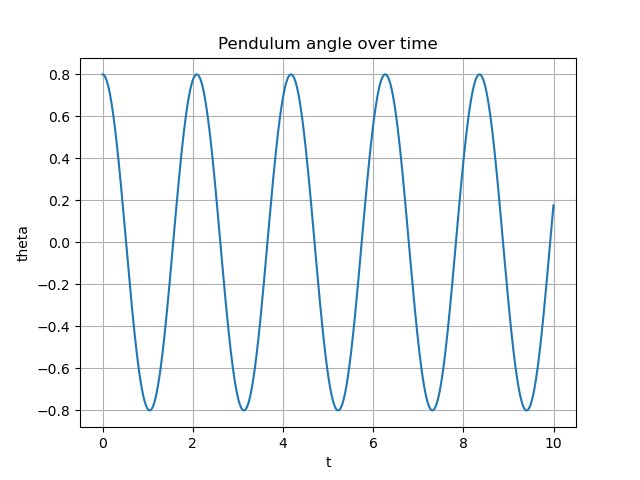
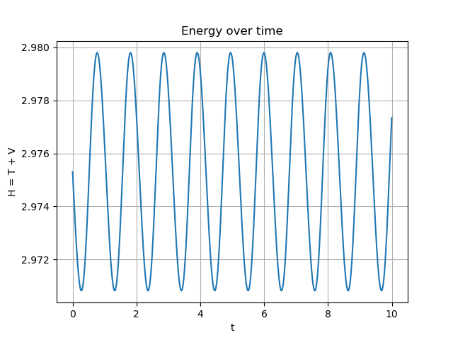
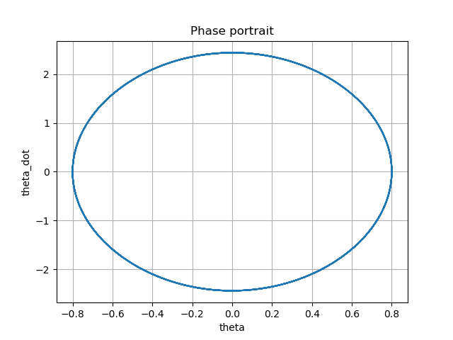
We see the pendulum rotates through the angles cyclically, and the energy is (roughly) conserved. So the code passes the basic sanity test.

Adding Lie Groups

The implementation above doesn’t actually use our Lie Group formulation. We should hook in our Lie Group library¹³.

We replace our discrete lagrangian code above with the following:

    def discrete_lagrangian(self, qk: torch.Tensor, qk1: torch.Tensor, h: float) -> torch.Tensor:

        mid_coords = []
        vel_coords = []

        for name, (group, sl) in self.model.layout.items():
            qk_i  = qk[sl]      
            qk1_i = qk1[sl]

            gk  = group.exp(qk_i)
            gk1 = group.exp(qk1_i)

            omega = group.log(gk.inverse() * gk1) / h        
            g_mid = gk * group.exp(0.5 * h * omega) # equivalent of midpoint quadrature 

            mid_i = group.log(g_mid)   
            vel_i = omega             

            mid_coords.append(mid_i)
            vel_coords.append(vel_i)

        mid = torch.cat(mid_coords, dim=-1)
        vel = torch.cat(vel_coords, dim=-1)

        ctrl  = self.model.unpack(mid)   
        dctrl = self.model.unpack(vel)   

        return h * self.lagrangian(ctrl, dctrl)

In the purely Euclidean case, with \(q_k, q_{k+1} \in \mathbb{R}^n\), the discrete Lagrangian I used is just the midpoint rule applied to the action integral. That is:

\[ L_d(q_k, q_{k+1}; h) := h\,L\!\left(q_{k+\tfrac12}, \, v_k\right) \]

where

\[ q_{k+\tfrac12} := \frac{1}{2}(q_k + q_{k+1}), \qquad v_k := \frac{q_{k+1} - q_k}{h} \]

So the discrete action becomes

\[ \mathfrak{G}_d(q_0,\dots,q_N) = \sum_{k=0}^{N-1} L_d(q_k, q_{k+1}; h) = \sum_{k=0}^{N-1} h\,L\!\left( \frac{q_k + q_{k+1}}{2},\, \frac{q_{k+1} - q_k}{h} \right) \]

On a Lie group \(G\) (or a product of Lie groups), the “midpoint” and the “finite difference velocity” should be expressed in group and algebra coordinates.

Given local coordinates \(q_k, q_{k+1}\) in the Lie algebra \(\mathfrak{g}\), we interpret them as group elements via

\[ g_k := \exp(q_k), \qquad g_{k+1} := \exp(q_{k+1}) \in G \]

The group-relative increment from \(g_k\) to \(g_{k+1}\) is

\[ \Delta g_k := g_k^{-1} g_{k+1} \]

and its corresponding algebra element is

\[ \omega_k := \frac{1}{h}\,\log(\Delta g_k) = \frac{1}{h}\,\log\bigl(g_k^{-1} g_{k+1}\bigr) \;\in\; \mathfrak{g} \]

which plays the role of a discrete velocity.

A natural “midpoint” configuration is obtained by “flowing” halfway along this group velocity:

\[ g_{k+\tfrac12} := g_k \exp\!\Bigl(\tfrac12 h\,\omega_k\Bigr). \]

To feed this back into the Lagrangian \(\ell : \mathfrak{g} \to \mathbb{R}\) written in algebra coordinates, we take

\[ q_{k+\tfrac12} := \log(g_{k+\tfrac12}), \qquad v_k := \omega_k. \]

So the Lie-group discrete Lagrangian is

\[ L_d(q_k, q_{k+1}; h) := h\,\ell\!\left(q_{k+\tfrac12},\, v_k\right) = h\,\ell\!\Bigl( \log\!\bigl(g_k \exp(\tfrac12 h \omega_k)\bigr),\, \omega_k \Bigr), \]

with \(g_k = \exp(q_k)\) and \(\omega_k = \tfrac1h \log(g_k^{-1} g_{k+1})\).

When \(G = \mathbb{R}^n\) with its additive Lie group structure (so \(\exp\) and \(\log\) are both the identity), this reduces exactly to the Euclidean midpoint formula above.

For \(\mathbb{R}^n\), the Lie Groups are trivial and this reduces back to the original midpoint quadrature.

If we run the code we see:

Final Theta: 0.7583324173185618
Energy stats:
  min: 2.4167871253032307
  max: 2.975317957405105
  drift: -0.1006878866394163

Error is much worse. I suspect this is due to the _log_impl function in the SOn class (which is only a first-order approximation). This took some debugging to get to this point. There could easily be other issues, but I’m content to move on and look again only if I end up needing this library in the future.

Another issue is that the Lie Group wrappers really slow down the code. If we need to return to Lie Groups and the performance becomes a problem, I will optimize.

Conclusion

In this post, we built up some foundational understanding of geometric controls and Lie Groups/Algebras. We did this “geometrically” - our intuition is not derived from physics per se but from the relevant geometric abstractions.

I have a few other posts to complete before I come back to this topic, but I want to continue to pursue this line of reasoning in the upcoming year. This may include \(n\)-plectic control, Noetherian theorems, approximate Lagrangians, Morse theory, differential cohomology, etc. I’ll also hopefully begin to look at other systems from the geometric viewpoint (like thermodynamics). This is mostly based on a hunch that we can develop more intuitive and general abstractions for controls based on geometric principles, and that we can use these tools to gain some deeper physics insights into how agents function theoretically.

Additionally, I think that there’s low-hanging fruit in our discrete Lagrangian solver. There are three views we can use, that should all be equivalent: the Lagrangian (global optimization) view, the Hamiltonian (local policy) view, and the “black-box simulator” view. We should be able to build a minimal library that allows us to define a problem, develop a unified, abstract geometric representation, and then translate between the different views. There’s also something interesting about how we have dual views around the variables to be controlled and their gradients (perhaps there is something interesting we can do with autograd?). Hopefully we will also develop this further.

Footnotes

1. This brings us to the realm of differential geometry. I will attempt to explain and derive these principles purely geometrically, without any reference to physics.

2. We may be able to get away with less structure here than a Riemannian metric, probably just \(C^2\) with invertible Hessian and maybe positive definite (for the Hamiltonian). But let’s assume the full metric structure for now.

3. It’s interesting to consider what would happen if the Hamiltonian WAS multi-valued, or if we only had “approximate inverses” for some reason… maybe more on this in a future post (if I can figure it out).

4. For a general Lagrangian, the Legendre map is controlled by the Hessian of \(L\) in \(v\); the Riemannian metric is a special case where this Hessian comes from \(g_q\) (as in mechanical systems).

5. This seems arbitrary. Geometrically, this is like assuming the initial reference frame inside the robot is arbitrary - that is, modulo the initial position, the paths followed are “the same”. You can also assume right-invariance (which assumes the “outside observers” reference frame doesn’t matter). This is basically dual to the left-invariance case, the same but from the observers point of view. It might come up in tracking or estimation (controlling how you view a robot). If you assume both (bi-invariance), then neither position nor direction matter. This is like a assuming a perfectly round sphere in free space floatig in a featureless fog. If we don’t assume either invariance, then the Lagrangian depends on position, not just velocity. There is something external breaking the symmetry.

6. Differentiating in this way makes the implicit assumption that we have matrix Lie Groups. If we don’t make that assumption the upshot is we get a slightly more general formula for the Lie bracket (later). \([\omega, \eta] := \text{ad}_{\omega}\eta\).

7. The derivative of a smooth function \(\ell: \mathfrak{g} \to \mathbb{R}\) at a point \(\omega\) is a linear map \(d\ell_\omega: \mathfrak{g} \to \mathbb{R}\) — that is, a covector. So \(\mu = \frac{\partial \ell}{\partial \omega}\) naturally lives in the dual space \(\mathfrak{g}^*\).

8. Sign conventions in the literature sometimes differ by a minus sign. The adjoint map \(\operatorname{ad}_\omega: \mathfrak{g} \to \mathfrak{g}\) is defined by \(\operatorname{ad}_\omega(\eta) := [\omega,\eta]\). The coadjoint map \(\operatorname{ad}_\omega^*: \mathfrak{g}^* \to \mathfrak{g}^*\) is its dual (transpose) in the linear-algebra sense: for every \(\mu \in \mathfrak{g}^*\) and \(\eta \in \mathfrak{g}\), \((\operatorname{ad}_\omega^* \mu)(\eta) = \mu([\omega,\eta]).\) This is exactly what we used when we rewrote the term \(\mu([\omega,\eta])\) as \((\operatorname{ad}_\omega^*\mu)(\eta)\) in the variation.

9. Assumes \(\omega\) is constant in time.

10. It seems like the reason is that the velocity is already encoded in the differences between positions. This may merit more thought, especially if we progress to “higher-dimensional” Lagrangians, as I may do in a future post. I did not rederive the equation for the discrete Lagrangian for this post.

11. The signs seem to be flipped because in the discrete setting, we are varying the points themselves, which does not require integration by parts.

12. manif cites this paper in particular.

13. One important note: PyTorch doesn’t seem to offer matrix log, which led to a lot of weirdness around the \(SO_n\) implementation, that I didn’t want to focus too hard on, as it isn’t the focus of the post. Be careful with this code!