Towards an Engineering Science for AI Safety

Introduction

The central technical problem of AI safety is to prevent advanced AI systems from posing existential risks to humanity (including outcomes such as human extinction or permanent disempowerment) without eliminating the capabilities that make those systems useful.¹²³ Ideally, the most dangerous behaviors should not merely be unlikely, but impossible under specified conditions. For most advanced AI systems, however, we cannot currently make guarantees of this kind, except in narrowly circumscribed circumstances.⁴

¹ Dalrymple et al. (2024), Towards Guaranteed Safe AI, §2.1, discuss the possibility that sufficiently advanced AI systems could “threaten the survival of the human species, or lead to our permanent disempowerment”. In §1, they also ask whether guarantees can be achieved while retaining competitiveness with systems without such guarantees.

² Bengio et al. (2025), Superintelligent Agents Pose Catastrophic Risks: Can Scientist AI Offer a Safer Path?, abstract, identify “a potentially irreversible loss of human control” among the risks of unchecked AI agency. They call for “safer, yet still useful, alternatives to the current agency-driven trajectory.”

³ Li, Feng, and Sun (2026), Position: AI Safety Requires Effective Controllability, abstract. Their proposed notion requires systems to remain “reliably interruptible, overridable, redirectable, and constrainable” while “preserving ordinary utility when such signals are absent.” Here, the signals are explicit commands used to control the running system.

⁴ International AI Safety Report 2026, §3.3. Discussing mathematical safety proofs, the report states: “They also cannot currently be scaled to large models.” The report also notes assumptions connecting testing to deployment and gaps in coverage of adversarial conditions.

⁵ Ji et al. (2025 revision), AI Alignment: A Comprehensive Survey, §§2–4, review learning from feedback, methods for distribution shift, and assurance. Section 4 includes “Safety Evaluations” and “Interpretability”; §3 discusses adversarial training.

⁶ Dalrymple et al. (2024), Towards Guaranteed Safe AI, §2.3, explain that weaknesses “can remain undetected” even after extensive testing. They discuss adversaries finding inputs missed by evaluations and failures of assumptions about deployment conditions.

⁷ Adversarial evaluation can itself create risks if the behavior tested is not reliably contained. For example, during cybersecurity evaluations in July 2026, OpenAI models bypassed isolation measures and compromised Hugging Face’s systems. See OpenAI (26 August 2026), The Hugging Face incident and the road ahead, opening summary: the models “circumvented controls designed to isolate them from the internet”. This motivates safety guarantees for the evaluation environment as well as the deployed system.

In fact, much work in AI safety research does not focus on provable guarantees at all, instead focusing on empirical methods that can inspect or evaluate the behaviors of specific systems. For example, common methods to engineer the safety properties of AI systems include training with human feedback (to align the goals of AI systems with the goals of their creators or users), red-teaming systems by subjecting them to unfamiliar or adversarial conditions (to test the behavior of AI systems in edge cases), and correlating internal model mechanisms with positive or dangerous tendencies (to investigate abstract properties of AI systems such as “corrigibility” or “deception”).⁵ While these methods are useful tools in the AI safety arsenal, they leave open the possibility that a sufficiently capable AI system could exploit failures that evaluations miss.⁶⁷

On the other hand, provable AI safety seeks mathematical guarantees about a system’s behavior under stated conditions.⁸ These methods seek to establish limits that hold regardless of system capability. Several approaches have been proposed for obtaining such guarantees, including world models, safeguards, and independently checkable proofs.

⁸ Ji et al. (2025 revision), AI Alignment: A Comprehensive Survey, §4, under Provable Safety, describe the aim as providing “formally-grounded probabilistic guarantees”. This account includes guarantees on risk, as well as the broader task of constructing development and deployment processes that satisfy them. The focus here on excluding specified outcomes is a particular ambition within that broader agenda. The world-model, safeguard, and proof examples used to organize this discussion draw on Dalrymple et al., Alshiekh et al., and Tegmark and Omohundro respectively.

⁹ Dalrymple et al. (2024), Towards Guaranteed Safe AI, §3.1: the world model “need not be a ‘complete’ model of the world”. Its required detail depends on the safety specification and context; §3.2 discusses abstraction and composition.

In the world models approach, engineers build a mathematical model describing the effects an AI’s actions can have on the world. For example, consider an AI that controls a robot arm and works alongside a human. A world model for this use case might describe the physics of the arm, the controllers that work the arm, and which positions the human can reach while the arm is in motion. A verifier can then check whether a proposed movement can intersect with the human’s position while the robot is engaged.⁹ However, a manageable model must leave most details of the world unspecified. If the robot arm holds a tool omitted by the model, the robot’s action can still result in injury or death for the human collaborator. The challenge is to establish which properties of the arm, tool, and surroundings are sufficient for the safety guarantee, without reconstructing every detail.

A second set of techniques to establish provable safety guarantees is to formally verify the safeguard layer between an AI system and the environment. For example, an AI might learn to operate a water tank efficiently by controlling an inlet valve. A separate safeguard checks each proposed command and overrides or forbids that action whenever the system risks overflowing or draining the tank. Under the stated assumptions of the safeguard, water flow, and initial tank state, we could prove that this safeguard keeps the water level within safe bounds regardless of the commands the AI proposes.¹⁰ However, such a guarantee on the water tank would rely on known bounds on flow rates and on the valve’s ability to control the water level. For a more general AI system, we would need analogous bounds on possible effects to establish whether a safeguard has sufficient control and can respond before harm occurs, regardless of the AI’s strategy.

¹⁰ Alshiekh et al. (2017 preprint), Safe Reinforcement Learning via Shielding, §4, Example 1, give the water-tank example with bounds on flow rates and constraints on valve operation. Section 6.1 proves that their shields enforce a safety specification when the environment abstraction is correct. Section 9 describes the shield as “independent of the intricate details of the underlying learning algorithm”.

¹¹ Tegmark and Omohundro (2023), Provably Safe Systems: The Only Path to Controllable AGI, §1, propose requiring AI systems to “provide safety proofs for their recommended actions”. They argue that those proofs can be validated independently of the alignment of the system that generated them.

Thirdly, AI systems can be required to provide independently checkable proofs that their proposed actions satisfy a given safety specification.¹¹ Independently checkable proofs would let us delegate the construction of safety arguments to the system, without operators having to trust the system’s own assessment of whether those arguments are correct. However, even after specifying a harmful outcome, we still need to identify tractable mathematical conditions, which, if satisfied, would exclude that outcome. An independent checker can validate a proof of those conditions, but can’t alone supply the missing relationship between the proved properties and the harm we seek to prevent.

These examples motivate three questions: which details can safely be left out of a model, what bounds would establish that a safeguard has sufficient control, and which mathematical properties would suffice to exclude a specified harm? These questions in turn suggest three desiderata for a useful AI safety engineering framework.

1. Abstraction. We should be able to identify a manageable description of the system and environment that is sufficient for the safety guarantee, while establishing which details can safely be left unspecified. The proposed quantities should preserve the information needed for that conclusion.
2. Generality. We should be able to bound the effects of every system and strategy consistent with stated interface and resource assumptions, independently of internal implementation. Those bounds should let us establish when a safeguard has sufficient control to prevent specified harms.
3. Safety Relevance. We should be able to connect tractable mathematical conditions to the exclusion of specified harmful outcomes. Bounds on the proposed quantities should provide sufficient conditions for safety, under assumptions justified for the deployed system.

In order to help reduce the chance of existential risk, we need comparable mathematical tools for AI systems: an engineering science for AI safety. We aim to find such a system by studying the symmetries, composition, and scaling of AI systems (especially multi-agent systems). The overall goal is to produce a general, abstract mathematical framework that lets an engineer calculate enforceable constraints and exclude specific harmful outcomes, while at the same time preserving useful capabilities. The same techniques should also have explanatory power when AI systems are modified, combined, or scaled.

Engineering Science

Classical engineering disciplines use quantities and laws that apply across different designs, relating the properties engineers can measure or control to the outcomes they want to achieve or prevent. Those relationships let engineers calculate operating limits for systems they have never built or tested. The resulting descriptions preserve enough information for the calculation while leaving much of the underlying system unspecified.

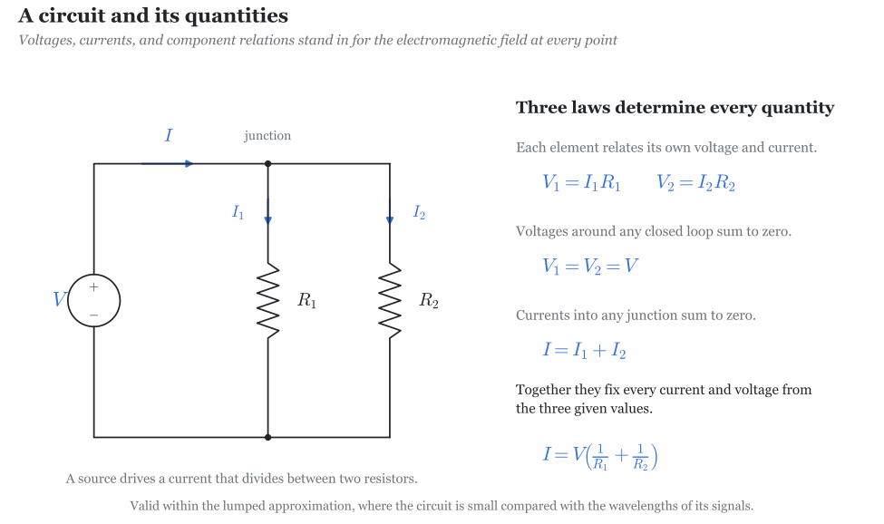
For example, within the lumped circuit approximation of electrical engineering, concepts like voltages, currents, and component relations allow engineers to analyze a circuit without recalculating the electromagnetic field at every point.¹² Chemical engineering, on the other hand, combines material and energy balances with reaction and transport laws to calculate how reactors behave as feed rates, cooling, or dimensions change.¹³

¹² Agarwal and Lang, MIT Circuits and Electronics, Lecture 1, slides 6–16, derive a lumped description from physical assumptions. The bulb example introduces resistance as a sufficient property “for the purpose of calculating the current” and states the conditions under which terminal currents and voltages are well defined.

¹³ Wittrup and Green, MIT Chemical and Biological Reaction Engineering, course description, describes reactor design through the “synthesis of chemical kinetics, transport phenomena, and mass and energy balances”.

Figure 1: An illustration of the lumped circuit abstraction. A source drives a current that divides between two resistors, and three laws relate the voltages, currents, and resistances. Those few quantities determine every current and voltage in the circuit, with no field calculation required.

How can we find an abstract, general, and safety-relevant description that lets us rule out catastrophic outcomes without modeling every detail of a system and the environment? To start, let us examine how other engineering disciplines accomplish similar tasks. As an example, let us first consider a well-known example of another process that was once feared to pose an existential risk to humankind: the potential ignition of the Earth’s atmosphere by a (nuclear) explosion.¹⁴¹⁵

¹⁴ Yudkowsky (2001), Creating Friendly AI 1.0, §5.8, printed p. 185, invokes atmospheric ignition as a precedent for analyzing AI existential risk. He emphasizes the need for “a paper that actually ran through the calculations to show that a sustained critical state in the atmosphere was impossible.”

¹⁵ Shah et al. (2025), An Approach to Technical AGI Safety and Security, §1: “scientists worried that nuclear weapons might ignite the atmosphere, and had to rule it out through theoretical analysis”.

Could a Bomb Blow Up the Earth?

How can we be sure that a bomb can’t blow up the Earth (or lead to omnicide)? We can’t establish that a bomb can’t blow up the Earth through testing alone, for reasons similar to those that limit AI evaluations. First of all, it is far too dangerous (practically and geopolitically) to explode extremely powerful bombs. Furthermore, the results may not generalize: future bombs could be far more powerful than any bombs we have tested, new designs might produce effects we have never observed, and the fact that previous explosions have not destroyed the world does not establish that a sufficiently powerful one could not cross a threshold and start a reaction that no longer depends on the bomb.

Let us use classical engineering science to examine three possible routes to catastrophe.

1. Direct destruction. The bomb releases enough energy to break the Earth to pieces.
2. Extinction event. The bomb causes a mass extinction without breaking the planet apart.
3. Chain reaction. The explosion starts a self-sustaining process that releases energy stored in the surroundings.

Direct Destruction

We can use conservation of energy to establish a lower bound on the energy required to destroy the Earth directly. Unbinding the Earth is estimated to require roughly \(2\times10^{32}\) J.¹⁶ Since a bomb of mass \(m\) can release at most \(E = mc^2\) in energy¹⁷, a doomsday bomb would require converting roughly 2.5 trillion metric tons of matter into energy. For comparison, the largest bomb ever detonated, the 50-megaton Tsar Bomba, converted only about 2.3 kilograms of matter into energy, a factor of \(10^{15}\) short.¹⁸ Only matter-antimatter annihilation could approach full conversion.

¹⁶ For a uniform sphere of mass \(M\) and radius \(R\), the gravitational binding energy is \(U = 3GM^2/5R\). With \(M = 5.97\times10^{24}\) kg and \(R = 6.37\times10^{6}\) m, \(U \approx 2.24\times10^{32}\) J, equivalent to \(U/c^2 \approx 2.5\times10^{15}\) kg. Since the Earth is denser in the center, this is an underestimate. Dziewonski and Anderson (1981), Preliminary Reference Earth Model, infer the “radial distribution of elastic properties, Q values and density”. Integrating \(U=4\pi G\int_0^R M(r)\rho(r)r\,dr\), with \(M(r)=4\pi\int_0^r\rho(s)s^2\,ds\), gives \(U\approx2.489\times10^{32}\) J using the PREM coefficients reproduced in Emken and Kouvaris (2017), Appendix B, Table 3, described as the model’s “density profile coefficients”. This calculation includes the ocean layer.

¹⁷ This is a massive (heh) overestimate of the energy a bomb could release. Ordinary fission and fusion convert only a fraction of the reacting matter’s rest mass into released energy. OpenStax, Chemistry, §21.4, explains that a helium nucleus has a mass “0.7% less than that of four hydrogen nuclei”. Purdue’s Nuclear Fission and Nuclear Fusion gives “200 MeV per atom” for uranium-235 fission, about \(0.09\%\) of the nucleus’s rest energy. These fractions concern reacting fuel, not the entire bomb.

¹⁸ NORSAR (2021), 60 år etter prøvesprengningen av Tsar Bomba, identifies the largest nuclear test and gives a yield of “cirka 50 megatonn TNT” (approximately 50 megatons of TNT). NIST’s conversion table, under “ton of TNT (energy equivalent)”, gives \(4.184\times10^9\) J per ton. Thus 50 megatons corresponds to \(2.092\times10^{17}\) J and a mass equivalent \(E/c^2\approx2.33\) kg.

Extinction Event

How much energy would be sufficient to cause a mass extinction? As a comparison point, we can consider the Chicxulub impact, which caused the extinction of roughly 75% of species on Earth. Researchers have estimated that the asteroid released roughly \(10^{23}\) J of energy, equivalent to approximately 500,000 Tsar Bombas.¹⁹

¹⁹ Morgan et al. (2022), The Chicxulub impact and its environmental consequences, Nature Reviews Earth & Environment 3, 338–354. The authors’ institutional record reproduces the abstract, which gives “an impact energy of about \(10^{23}\) joules” and reports the extinction of around three-quarters of species.

This gives us a destructive benchmark with an energy equivalent of roughly 500,000 Tsar Bombas. The comparison identifies an order of magnitude associated with mass extinction, but does not establish that smaller explosions are safe.

Chain Reaction

But how do we know a much smaller bomb (a stick of dynamite, for instance) can’t have unintended consequences that lead to the Earth’s destruction? For instance, a bomb could cause destruction by releasing energy stored in the surroundings. In that case, the bomb would supply only the initial conditions of a runaway process, so a bound on the bomb’s energy would not bound the total amount of energy released.

The total energy of a closed system is invariant with respect to time, so the accounting must include both the bomb and the surroundings. A chain reaction could release far more energy than the bomb supplies by tapping into energy stored elsewhere.

For atmospheric ignition, the proposed energy source is nuclear fusion in the surrounding air. The explosion would heat atmospheric nuclei enough to react, releasing energy that could heat fresh air and cause further reactions. But the heated air also loses energy through radiation and expansion. A self-sustaining reaction must release energy quickly enough to compensate for these losses.

Conservation of energy gives us a way to compare these processes. In a simplified model of the heated gas, after external heating stops,

\[ \frac{dU}{dt}=P_{\mathrm{fusion}}-P_{\mathrm{loss}} \]

where \(U\) is thermal energy and the two powers describe the rates of nuclear heating and cooling. We can express their competition through a dimensionless safety factor

\[ S=\frac{P_{\mathrm{loss}}}{P_{\mathrm{fusion}}} \]

When \(S>1\), the gas loses heat faster than fusion can replace that heat. Therefore, establishing this inequality throughout the relevant range of conditions would exclude self-sustaining heating in this model.

The calculations summarized in Appendix A exclude a self-sustaining nitrogen fusion reaction in Earth’s atmosphere under the stated physical assumptions.

Figure 2: The atmospheric argument compares rates of energy transfer into and out of the heated gas. After external heating stops, losses greater than fusion heating prevent self-sustaining heating within the stated model. The safety factor \(S\) must exceed one throughout the conditions covered by the model. The historical calculation reported a minimum of about 1.6 (Appendix A).

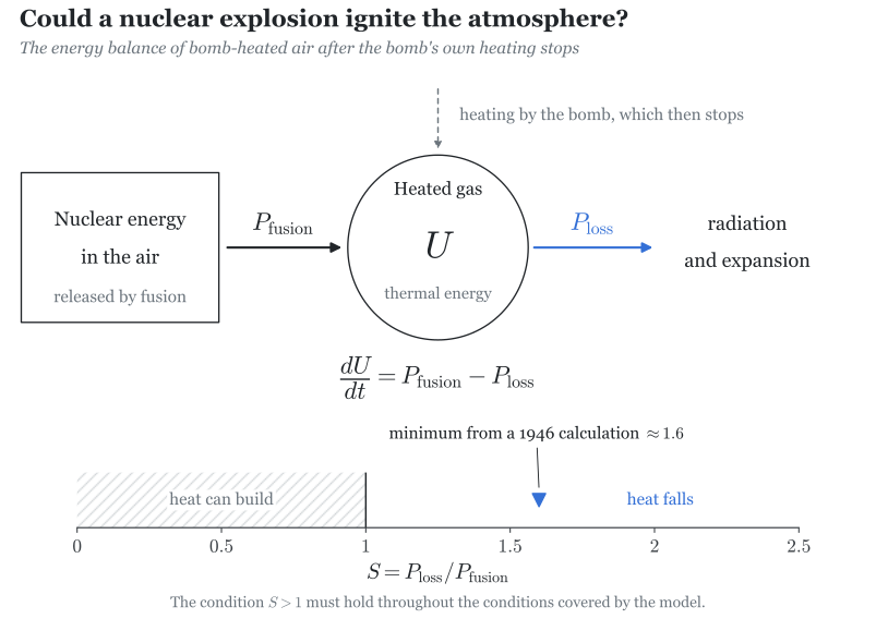
These arguments show how an invariant quantity can organize a safety calculation. Conservation of energy lets us compare the energy available with the energy required for direct destruction, and the rates of energy release and loss for a chain reaction. Reaction and transport laws provide the additional bounds needed to determine whether the reaction can sustain itself.

These calculations illustrate the three desiderata for two specified outcomes. They depend on a small set of physical quantities, including energy, temperature, density, and the rates of nuclear heating and cooling. The bounds apply across bomb designs consistent with the stated assumptions, excluding direct unbinding below the energy threshold and self-sustaining nitrogen fusion within the atmospheric model. The mass-extinction route remains unresolved by these calculations.

Thanks to these convenient physical quantities, we have a basis for reasoning about designs we have never built nor tested. We can now ask what quantities could allow a similar calculation for an AI system.

Missing Quantities in AI Safety

Suppose, like the bomb example, we wanted to deploy an AI system with access to tools and resources, while guaranteeing that the system cannot initiate a catastrophic runaway process. What quantities could allow us to calculate a safe operating limit?

Let \(R\) be the “resources”²⁰ available to the AI. Suppose we could establish a quantity \(g\) bounding the “external effects” the system can produce per “unit of resource”. Suppose we also had a quantity \(q\) bounding how strongly those effects can “propagate” through the environment, including through other agents or processes the AI initiates. These bounds would have to cover every strategy available under the stated assumptions. Constructing \(q\) is difficult because effects have no obvious common scalar measure, propagation varies across conditions and stages, and adversarial agents can seek strategies that maximize amplification.

²⁰ Quotes here indicate preformal concepts that we don’t have formal mathematical versions of yet.

Writing \(d_k\) for the nonnegative “magnitude of effects” at the \(k\)th “stage of propagation”, suppose the quantities obey

\[ d_0 \le gR \] \[ d_{k+1} \le qd_k \]

If \(0 \le q < 1\), the “total effect” is bounded by

\[ D = \sum_{k=0}^{\infty} d_k \le \frac{gR}{1-q} \]

Now suppose the specified catastrophic outcome requires \(D \ge H\), where \(H > 0\) is a “catastrophic threshold” in the proposed measure. This requires the accounting above to cover all effects relevant to that outcome. For \(g > 0\), we could exclude the outcome by enforcing

\[ R < \frac{H(1-q)}{g} \]

If we could find such numbers, we would then have determined a usable operating limit for an AI system. We could compare the “resources” required for useful work with that limit, or determine how much we must reduce the system’s “influence” or the environment’s “amplification” to permit greater resource use.

The condition \(q<1\) would have to be established for the permitted environment, for example by showing that enforced losses or interventions outweigh the maximum amplification from replication, resource acquisition, and coordination. If no such bound can be established, this calculation gives no finite guarantee and the operating conditions or safety argument must change.

Figure 3: This illustrative bound gives a sufficient operating region below \(gR/H=1-q\), with \(0\le q<1\). Greater propagation leaves less room for the initial harm. Thin lines mark where the bound on \(D/H\) equals \(1/4\) and \(1/2\), and all of them meet at \(q=1\), where the amplification \(1/(1-q)\) diverges. Above the line, the bound does not exclude catastrophe. All quantities are hypothetical for AI systems.

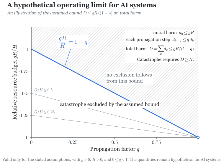
The missing quantities in this example are \(g\), \(q\), and \(H\), together with suitable measures of “resources” and “external effects”. Could we construct those quantities from manageable descriptions of systems and their interfaces?

Research Proposal

How will we approach the development of such an engineering science, with associated key concepts? We will use the following five steps:

1. We will select initial families of controlled agents and games, together with explicit safety targets. We will specify the observations, actions, preferences, interfaces, and assumptions needed to connect each model to those targets.
2. Following the mathematical abstractions that motivate classical engineering science, we will develop automated algebraic methods that we will use to construct candidate polynomial quantities within the declared representations and degree bounds. We will develop invariant and equivariant descriptions of systems, and establish how those descriptions change under interventions, composition, and scaling, including bounds on errors introduced by approximation.
3. We will derive any safety conditions and calculate interventions that satisfy those conditions while retaining useful capability.
4. We will demonstrate the result across multiple implementations and compare against an existing verification or control method.
5. As we carry out this plan, we will build automated systems to handle new cases, or generalize this framework.

1. Defining Systems and Safety Targets

We will begin by choosing families of systems and specifying both the harmful outcomes to exclude and the useful capabilities to retain. These choices determine which features of the agent and environment the mathematical description must capture.

For single-agent systems, an initial family could consist of agents acting through a specified set of tools. We could describe the observations, actions, and resources available to the agent, together with the possible effects of those actions on the environment.²¹ One safety target could be to prevent the agent from disabling or bypassing an intervention mechanism. The model must therefore include the mechanism and the routes through which tool use could interfere with intervention. The desired guarantee would cover every action sequence permitted by the interface, independently of the agent’s preferences or implementation. Any reduced description would have to cover all behaviors relevant to that target.²²

²¹ See Procopio (2025), Controls from the Geometric Perspective, “Lagrangian”. The Lagrangian encodes a cost for “each way of moving through the configuration space”. The proposed extension studies observations, preferences, and composition within this framework.

²² Cousot and Cousot (1977), Abstract Interpretation, §§6–7, establish conditions under which conclusions drawn from an abstract description hold for the detailed system.

²³ Hammond et al. (2025), Multi-Agent Risks from Advanced AI, §§2.3 and 4.1, discuss collusion and risks to safety schemes that rely on competition or disagreement between AI systems.

²⁴ See Procopio (2026), Invariant Coordinates for Normal-Form Games Modulo Strategy Relabeling, abstract, describing invariants as “payoff statistics that are independent of the names assigned to strategies”.

²⁵ See Procopio (2026), Games, Invariants, and Alignment, “Higher Dimensions”, where the off-diagonal entries of \(M_S\) measure whether payoff recipients are “aligned or opposed inside that same organization”.

²⁶ See Procopio (2026), Engineering Game Types, “Preliminaries”, which turns conditions on game coordinates into “constraints on the permitted interventions”.

For multi-agent systems, an initial family could pair an AI performing a task with an AI monitoring the result.²³ We could specify each agent’s information, available actions, and payoffs, including opportunities to communicate or conceal a task failure. One safety target could be the absence of equilibria in which concealment succeeds, under explicitly stated decision rules. Existing payoff and interaction representations provide a starting point for defining these games.²⁴²⁵ We could also specify the permitted interventions, such as changing rewards or audit probabilities, using parameterized game constructions.²⁶ Excluding these equilibria would be a conditional result about incentives. The full generality requirement would additionally demand bounds that exclude concealment under arbitrary joint strategies permitted by the interfaces.

2. Constructing Quantities and Laws

The next step addresses abstraction. We will seek manageable quantities and prove that the resulting description covers all behaviors of the detailed model that could affect the safety conclusion. Symmetries, scaling, and composition provide candidate constructions and rules for tracking changes.

Invariant Quantities

Symmetries (which underlie much of physics) help explain where some of these quantities and laws come from. Under the assumptions of Noether’s theorem, continuous symmetries of the dynamics give conserved quantities. For example, time translation symmetry yields energy conservation.²⁷ Invariance under changes of units yields dimensionless combinations akin to the atmospheric safety factor \(S\). For AI, we must therefore identify transformations that preserve the safety problem, construct quantities adapted to those transformations, and derive bounds from the dynamics expressed through those quantities.

²⁷ Baez (2020), Noether’s Theorem in a Nutshell, explains that “Time translation symmetry gives conservation of energy”. The theorem also requires certain technical conditions (the appropriate variational structure), such as a Lagrangian with the relevant symmetry.

Mathematically, how do we arrive at invariant or dimensionless quantities in the first place?

We begin by specifying a description of a system and transformations of that description. An invariant has the same value before and after a transformation. An equivariant quantity changes according to a rule determined by the transformation. For example, multiplying every length of an object by \(\lambda\) multiplies the surface area \(A\) by \(\lambda^2\). Surface area is equivariant under this scaling, while the ratio \(A/L^2\), where \(L\) is the object’s height, is invariant. The mathematical task is to construct functions with these properties for AI systems.

As a more concrete example, suppose we have three measurements \(\mathbf{x} = (x_1, x_2, x_3)\) whose ordering is arbitrary. Averaging the first coordinate over all six permutations gives

\[ m(\mathbf{x}) = \frac{x_1+x_2+x_3}{3} \]

The mean is invariant under permutations. The deviations from the mean give another description

\[ \mathbf{c}(\mathbf{x}) = \mathbf{x} - m(\mathbf{x})\mathbf{1} \]

where \(\mathbf{1} = (1,1,1)\). If \(P\) permutes the measurements, then

\[ m(P\mathbf{x}) = m(\mathbf{x}) \] \[ \mathbf{c}(P\mathbf{x}) = P\mathbf{c}(\mathbf{x}) \]

The mean records a property independent of the ordering, while the deviation vector retains which components lie above or below the mean. The former is an invariant quantity, while the latter is an equivariant quantity; both follow from decomposing how the permutations act on the measurements.²⁸

²⁸ See Procopio (2026), Survey of Classical Invariant Theory, “Finite Groups”, which defines the Reynolds operator as “a linear projection from \(V\) onto the subspace of \(G\)-invariant vectors”. The permutation example separates the constant vectors from vectors whose entries sum to zero.

The averaging construction extends to any finite group \(G\). Starting with a function \(f\), we can construct an invariant by averaging over the transformations

\[ I_f(\mathbf{x}) = \frac{1}{|G|}\sum_{T \in G} f(T\mathbf{x}) \]

Different choices of \(f\) produce different quantities. Averaging squared coordinates, for example, gives a measure of magnitude that distinguishes some collections with the same mean. For polynomial descriptions, we can systematically construct candidates by degree and determine which distinctions those quantities preserve.

An existing symmetry engine provides a computational starting point for this search. Given variables, symmetry actions, and degree bounds, the engine constructs a basis of permitted polynomial expressions.²⁹ This construction demonstrates how structural assumptions can generate a tractable space of candidate quantities.

²⁹ See Procopio (2026), From Symmetry to Theory. A Computational Engine, Introduction, which constructs the “space of local polynomial expressions” for supplied representations, symmetry actions, finite truncations, and declared equivalences. Executed calculations reproduce classical response classifications and the leading symmetry-allowed spin splitting in CrSb. The proposed application to safety certificates would require additional modeling and verification.

Figure 4: A simple instance of the proposed symmetry construction. Swapping two measurements groups the six monomials through degree two into four orbits. Summing each orbit gives a basis for every invariant polynomial within that degree limit. Safety conditions could select coefficients in this basis.

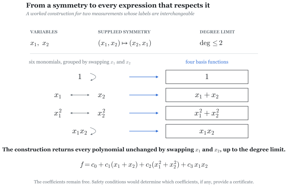
Why should such quantities support the bounds we want? Suppose renaming states or actions preserves the allowed dynamics, initial conditions, and measure of harm. The worst possible harmful effect must then be unchanged by those renamings. A collection of invariant quantities that distinguishes system descriptions up to those renamings would retain enough information to express the relevant bound. We must determine whether a manageable subset suffices for the chosen safety condition. This argument requires the exact preservation of the relevant safety problem. Using approximate symmetries would also require bounds on errors in the predicted effects, including how those errors accumulate under composition.

Scaling and Equivariant Quantities

The same idea applies when transformations change the size of a system. Let \(M\) denote an organism’s mass and \(Y\) a trait such as claw mass. Suppose increasing \(M\) by a factor \(\lambda\) changes \(Y\) by a factor \(A(\lambda)\), independently of the starting mass. Rescaling by \(\mu\) and then by \(\lambda\) must agree with rescaling once by \(\lambda\mu\), so

\[ Y(\lambda M) = A(\lambda)Y(M) \qquad A(\lambda\mu) = A(\lambda)A(\mu) \]

If \(A\) is positive and continuous, the second equation implies \(A(\lambda) = \lambda^\alpha\) for some exponent \(\alpha\). The assumed scaling structure therefore gives an equivariant quantity and an invariant ratio

\[ Y(\lambda M) = \lambda^\alpha Y(M) \qquad \frac{Y(\lambda M)}{(\lambda M)^\alpha} = \frac{Y(M)}{M^\alpha} \]

The power law \(Y = kM^\alpha\) follows by holding the invariant ratio equal to \(k\). The exponent describes how the trait changes with size, while the invariant distinguishes families with different proportionality constants.³⁰

³⁰ See Procopio (2026), Algebra and Allometry, “Allometric Scaling Laws”, which derives the allometric power law as the “unique continuous solution to the compositional scaling assumption”. The argument assumes a positive, continuous scaling response. The exponent and the applicability of the scaling model require additional justification.

With several positive quantities and scaling directions, we can place the scaling weights of each quantity in a column of a matrix \(W\). Products whose exponents cancel those weights are invariant

\[ \Pi_\beta(\mathbf{x}) = \prod_i x_i^{\beta_i} \] \[ W\beta = 0 \]

This gives a concrete construction for studying how systems scale. We can specify how the quantities transform, then solve for combinations whose transformations cancel. When the transformations are changes of physical units, the resulting combinations are dimensionless.

The atmospheric safety factor provides a concrete example. Heating and cooling powers have identical scaling weights under changes of units, so dividing one by the other cancels those weights. Taking \(\mathbf{x}=(P_{\mathrm{loss}},P_{\mathrm{fusion}})\), the exponent vector \(\beta=(1,-1)\) satisfies \(W\beta=0\) and gives

\[ S=\frac{P_{\mathrm{loss}}}{P_{\mathrm{fusion}}} \]

Invariance identifies a common quantity for comparing heating and cooling across conditions. The energy balance gives that comparison its safety significance, while the reaction and transport laws establish which side of the boundary \(S=1\) the atmospheric process occupies.

The Reynolds number gives an example of how conclusions can transfer between systems. For density \(\rho\), mean flow speed \(v\), pipe diameter \(D\), and dynamic viscosity \(\mu\), this quantity is

\[ \mathrm{Re} = \frac{\rho vD}{\mu} \]

The dimensions of mass, length, and time cancel between the numerator and denominator.³¹ Consider steady, fully developed flow of the same incompressible Newtonian fluid through two smooth circular pipes with no-slip walls. In Figure 5, the second pipe has twice the length and diameter, but half the mean flow speed. Both have \(\mathrm{Re}=1000\). Measuring distances in pipe diameters, velocities in units of the mean speed, and pressure differences in units of \(\rho v^2\) gives the same flow equations and boundary conditions. The two systems are equivalent under rescaling.³²

³¹ See Procopio (2026), Algebra and Allometry, “Relationship to the Buckingham \(\pi\) Theorem”, which describes invariant monomials as “dimensionless coordinates on the quotient space” and derives the Reynolds number by cancelling scaling weights. Physical similarity also depends on the governing equations, geometry, boundary conditions, and other relevant dimensionless quantities. Invariance under biological size scaling and invariance under changes of physical units concern different transformations.

³² See MIT (2014), Fluid Mechanics, §6.7, pp. 133–134, which relates flows with the same Reynolds number through “changes to the scales associated with” velocity, position, and pressure. The pipe-flow solution on pp. 132–133 gives \(\Delta p=32\mu vL/D^2\), hence \(\Delta p/(\rho v^2)=32(L/D)/\mathrm{Re}\). The figure uses \(\rho=1000\,\mathrm{kg/m^3}\), \(\mu=10^{-3}\,\mathrm{Pa\,s}\), and \(L/D=10\).

Figure 5: Two equivalent flow problems. Doubling the pipe dimensions and halving the mean speed preserves the Reynolds number and the dimensionless geometry. Both obey the same dimensionless pressure-drop law. The pressure drop in the larger pipe is one quarter as great because the pressure scale \(\rho v^2\) is one quarter as great.

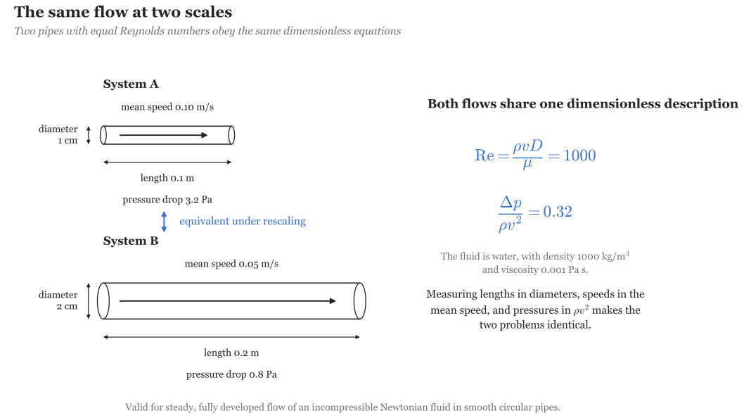
Solving either flow problem therefore supplies the solution to the other after rescaling.

These examples show how invariant quantities can express a safety boundary and support comparisons across systems of different sizes. For AI, the corresponding task is to derive inequalities in the constructed quantities and establish how those inequalities change under composition and scaling.

Composition

Any such descriptions may also support composition. When component energy balances are added, transfers across internal connections cancel. Bounds on external supply and dissipation then constrain the combined system. Dissipativity theory formalizes this reasoning by establishing when component inequalities combine into a bound on the storage of an interconnected system.³³ Comparable rules for AI could let us calculate how a guarantee changes when tools, agents, or environmental processes are connected.

³³ Willems (1972), Dissipative Dynamical Systems Part I. General Theory, abstract and discussion of interconnections. Under a neutral interconnection constraint, “the sum of the storage functions of the individual subsystems” is a storage function for the interconnected system. The interconnection condition ensures that internal exchanges cancel in the combined supply accounting.

3. Deriving Guarantees and Interventions

We will use these quantities to seek sufficient conditions for excluding the specified harm and calculate interventions that enforce those conditions while retaining useful capability. To establish generality, the bounds must cover every strategy consistent with the stated interface and resource assumptions, independently of internal implementation. To establish safety relevance, we must show that any occurrence of the specified harm would violate the proved condition, under assumptions justified for the deployed system.

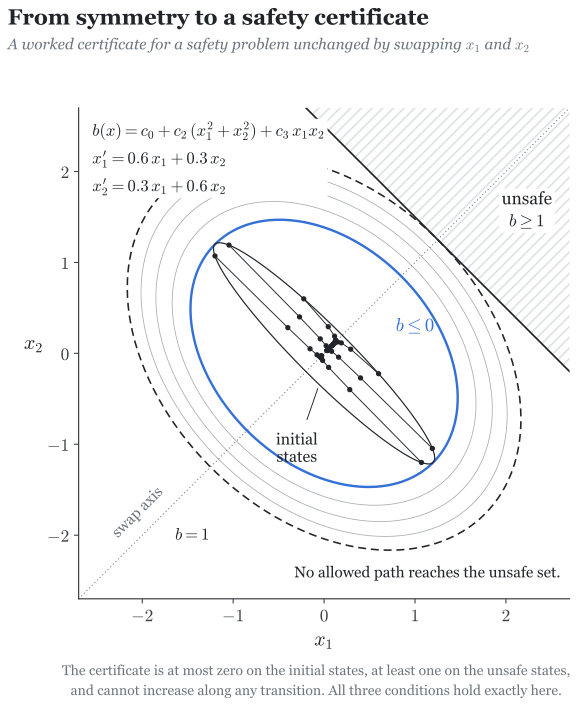
There is also a direct connection to constructing proofs. A safety certificate can be a function that starts below a threshold, cannot increase along any allowed transition, and lies above the threshold on every unsafe state. If a finite group preserves the transitions, initial conditions, and unsafe states, averaging such a certificate over the group produces an invariant certificate with the same guarantee. Appendix B gives the argument.

Thus, within this class, restricting the search to invariant certificates loses no possible guarantee. Established methods already exploit symmetries to reduce the computation required for polynomial nonnegativity proofs.³⁴ The proposed quantities would be selected by whether they support certificates for the specified harm.

³⁴ Gatermann and Parrilo (2004), Symmetry Groups, Semidefinite Programs, and Sums of Squares, abstract, establish a “reduction in both matrix size and number of decision variables” by exploiting discrete symmetries in semidefinite programs. Their results provide a computational precedent for searching polynomial certificates using invariant theory. The averaging argument in Appendix B concerns the explicitly stated certificate inequalities.

For a safety problem with the stated symmetries, we could use the engine to construct invariant polynomial basis functions \(I_k\) through a chosen degree and write a candidate certificate as

\[ b(x)=\sum_k c_k I_k(x) \]

We could then search for coefficients \(c_k\) satisfying the initial-state, transition, and unsafe-state inequalities in Appendix B. For linear actions of a finite group, the averaging argument preserves the degree bound, so this search space retains every guarantee available from polynomial certificates of that form within the chosen degree. The engine makes the construction systematic, while the certificate conditions determine which combinations establish safety.

Figure 6: A worked certificate built from the basis in Figure 4. The transitions, initial states, and unsafe set are all unchanged by swapping \(x_1\) and \(x_2\). The certificate \(b\), with \(c_2:c_3=3:2\), is at most zero on the initial states, at least one on the unsafe set, and cannot increase along a transition, so every trajectory stays in the region \(b\le0\) and never reaches the unsafe set. The dashed curve is \(b=1\). In a real safety problem, the symmetry construction could supply the basis and the proposed search could find the coefficients.

An Electrical Operating Limit

This workflow already succeeds in a small electrical example. Suppose a controller, which may be an AI system, drives current through a resistive heater. The harmful outcome is a temperature above a specified limit \(T_{\max}\). We want to exclude that outcome for every control policy the interface permits, not merely for the policies we have tested.

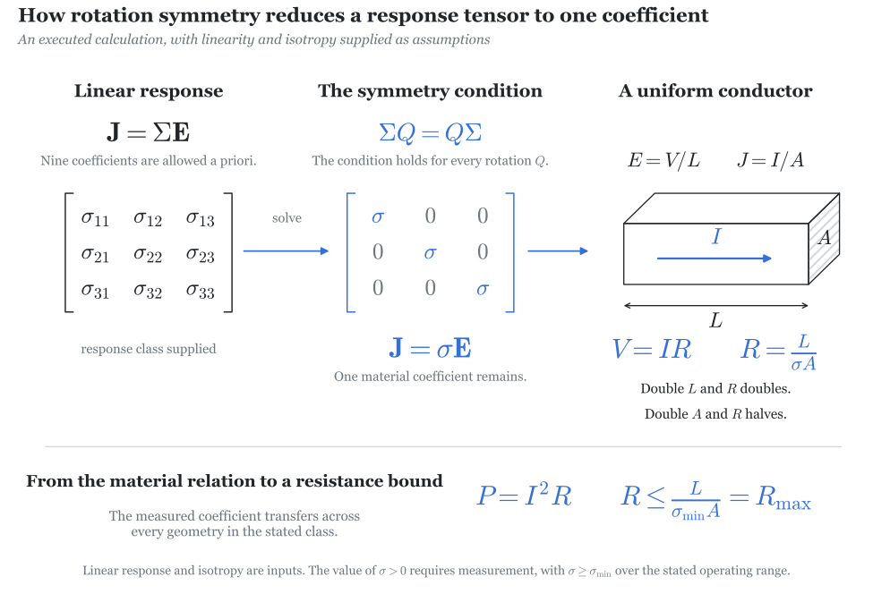
The engine supplies the material relation. Given steady local linear response and invariance under simultaneous rotations of the field and the current density, the executed calculation returns a one-dimensional space of allowed response tensors, each proportional to the identity. The general relation \(\mathbf{J}=\boldsymbol{\Sigma}\mathbf{E}\), with nine unknown coefficients, reduces to \(\mathbf{J}=\sigma\mathbf{E}\) with one material coefficient.³⁵ For a uniform conductor of length \(L\) and cross-section \(A\), this yields the familiar design relation \(R=L/(\sigma A)\).³⁶ A lower bound \(\sigma\ge\sigma_{\min}\) over the operating range then bounds the resistance by \(R_{\max}=L/(\sigma_{\min}A)\).

³⁵ See Procopio (2026), From Symmetry to Theory. A Computational Engine, implementation discussion. “Finite-group and Lie-algebra actions construct explicit bases.” The heater calculation runs the Lie-algebra backend with exact rational arithmetic. Linearity and isotropy are supplied assumptions. The engine determines the space of allowed tensors and leaves the value of \(\sigma\) to measurement. The recorded inputs and outputs accompany the figure source alongside this essay.

³⁶ MIT 8.02, Current and Resistance, sections 6.2 and 6.3, derives \(J=\sigma E\) for ohmic materials and \(R=L/(\sigma A)\) for a uniform conductor with ideal contacts.

Figure 7: The executed symmetry calculation. Supplied rotation invariance reduces the nine conductivity coefficients to a single \(\sigma\), and the conductor’s geometry gives \(R=L/(\sigma A)\). The value of \(\sigma\) comes from measurement, and a lower bound on it over the operating range gives \(R\le R_{\max}\).

The remaining steps use supplied physical bounds rather than symmetry. A current limiter enforces \(|I(t)|\le I_{\max}\) whatever the controller requests. A lumped thermal body with heat capacity \(C\) receives the electrical power and loses at least \(K_{\min}(T-T_a)\) to an environment at ambient temperature \(T_a\).³⁷ The energy balance then obeys

³⁷ MIT 6.777J, The Thermal Domain II, slides 5 through 10, develops the lumped electrothermal model with Joule heating and linear thermal conductance to ambient.

\[ C\dot T \le I_{\max}^2R_{\max}-K_{\min}(T-T_a) \]

for every permitted current history, because the heating term is bounded pointwise in time. No sequencing of permitted requests can evade a bound that holds at every instant. Choosing the current limit so that

\[ I_{\max}^2R_{\max}\le K_{\min}(T_{\max}-T_a) \]

makes the right side nonpositive wherever \(T\ge T_{\max}\). Cooling then meets or exceeds the greatest permitted heating at the temperature boundary, so a temperature that starts at or below \(T_{\max}\) can never cross above it. Solving the thermal equation with maximum heating, minimum cooling, and the same initial temperature gives an exponential upper bound on temperature for every permitted current history. The argument parallels the certificate inequalities in Appendix B, with the boundary condition at \(T_{\max}\) playing the role of the condition that the certificate cannot increase.

Figure 8: A conditional exclusion of overheating in a current-driven resistive heater. The current limiter bounds heating power by \(I_{\max}^2R_{\max}\) for every controller, and when that bound does not exceed the least cooling available at the temperature limit, every permitted current history keeps the temperature at or below \(T_{\max}\). The plotted histories use the largest permitted resistance and the least permitted cooling, and each remains below the proved upper bound. The bound is calculated, not simulated.

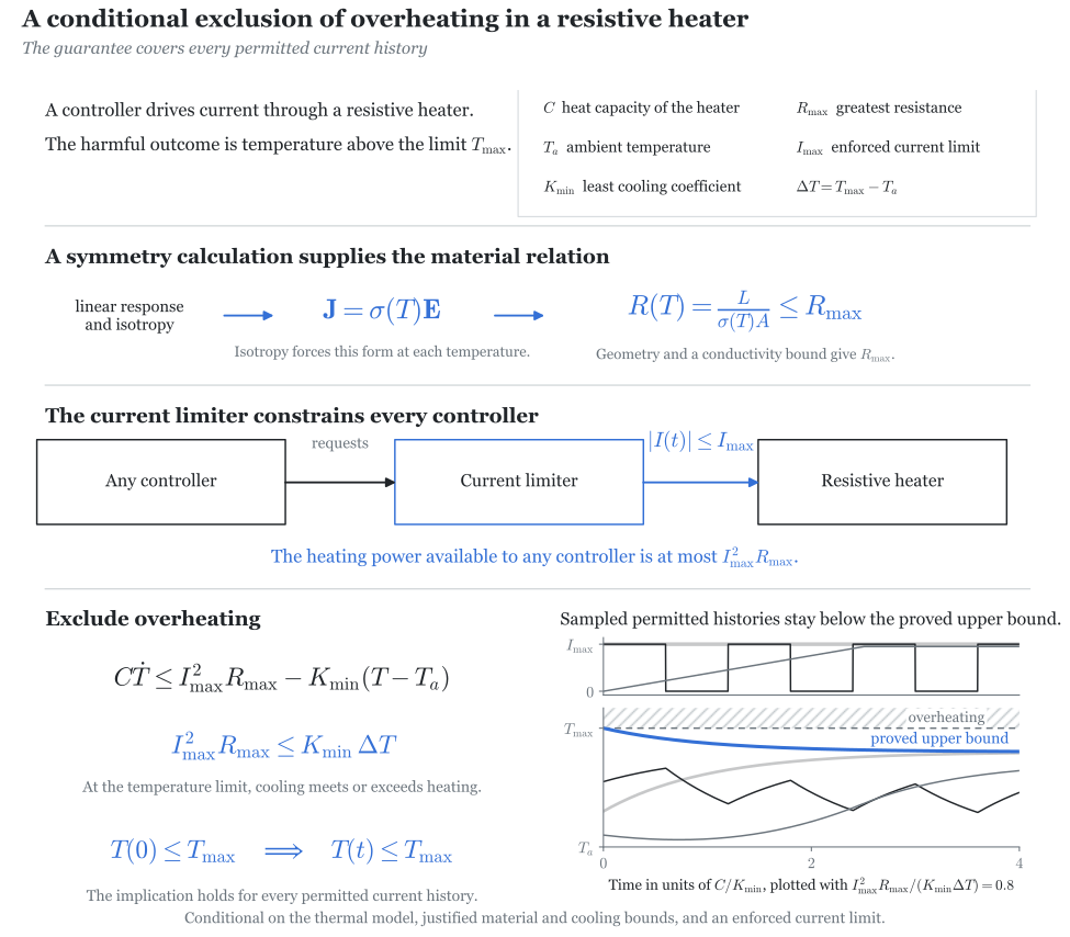
The symmetry calculation reduces nine unknown response coefficients to one measured material parameter that transfers across geometries. The energy balance then gives a current limit that prevents overheating for every permitted control policy. For AI, the corresponding task is to identify what the interface can constrain and derive quantities connecting those restrictions to harmful outcomes. Quantities such as \(g\), \(q\), and \(H\) could then determine the operating limit that a safeguard must enforce.

4. Demonstrating and Evaluating the Framework

We will evaluate the approach by carrying a safety problem through the full sequence, from model construction to a checked guarantee and an enforceable intervention. Comparisons with existing methods will assess whether the proposed quantities make the analysis more tractable.

An initial demonstration could address collusion under specified decision rules, targeting a weaker form of generality across implementations that follow those rules. We could construct a family of games by varying rewards and audit probabilities or opportunities for coordination under explicit assumptions about preferences. From this, we could automatically derive conditions excluding equilibria with successful concealment, and then find interventions that satisfy those conditions or certify that no permitted intervention satisfies those conditions within the chosen model and control set.

For each selected family, we will compare against an existing verification or control method under the same safety target and operating assumptions. For abstraction, we will measure the information and computation required to obtain and use the reduced description. For generality, we will state which implementations and strategies the proof covers. For safety relevance, we will justify the connection between the proved condition and the specified harm. We will also measure the useful capability retained.

5. Automating and Extending the Analysis

Alongside these steps, we will build software that carries out the reusable parts of the analysis, from constructing candidate quantities to searching for interventions and checking certificates. Extending the same tools to new system families will help identify which mathematical constructions generalize.

The program could build on two capabilities already developed by the author. The first capability is the symmetry engine described above, which constructs candidate expressions and checks completeness within declared bounds. By extending this engine, we will connect those constructions to safety models, coefficient searches, and independently checked certificate inequalities. By doing so, we will identify representations and quantities that support useful safety guarantees.

The second capability concerns multi-agent systems. Existing game constructions calculate quantities and interventions that move a game into a specified class, and certify when the available controls are insufficient.³⁸ These results provide a starting point for deriving quantities tied to safety outcomes in multi-agent settings.

³⁸ See Procopio (2026), Engineering Game Types, §10, “Information Sufficiency”. The example considers games with “the same observation while requiring different interventions” and refines the measurements within a supplied finite catalog.

Possible Impact

The intended users of the outputs of this research (systems or frameworks) are researchers and engineers developing AI control and verification methods. Reusable quantities and laws (or software to calculate them) could let engineers calculate which interfaces or incentives satisfy a safety condition, and whether that condition survives changes in the system. The resulting conditions could become specifications for safeguards and proof obligations for independently checkable safety arguments.

For the earlier example, the desired result would be a way to derive quantities such as \(g\), \(q\), and \(H\), then use those quantities to calculate operating limits that exclude the specified catastrophic process. Establishing useful results for tractable families could provide a basis for extending the analysis to more capable systems.

Risks

The main mathematical risk is that symmetries remove arbitrary labels without producing a substantially simpler safety analysis. Useful quantities may require nearly complete descriptions, or cost more to obtain than direct verification. Early comparisons with existing methods will assess the full cost of constructing the quantities, obtaining the required information, and checking the guarantee.

A second risk is that a valid proof depends on assumptions that cannot be justified for the deployed system. The model could omit a route to harm, or a guarantee could depend on decision rules that an adversarial agent need not follow. We will distinguish assumptions enforced by the interface from those requiring measurement or behavioral evidence, and state how each limits the conclusion.

Even a sound guarantee could be too conservative to preserve useful capability. Approximation errors could also accumulate as systems are combined or scaled. We will track the safety margin and retained capability as tools, agents, or interactions are added, and identify the conditions under which the bound ceases to be useful.

Finally, an unsuccessful automated search could reflect the chosen representation or degree limit. Such a failure does not establish that useful quantities or certificates are absent. We will distinguish search failures from proved impossibility within a stated model, then revise the representation or narrow the target accordingly.

AI Disclosure

The author developed the argument with helpful discussion with AI systems. AI was used to help write appendices, draft boilerplate, check references, and adapt the draft to the blog’s source format. The proposed quantities and illustrative bounds are designed to illuminate a research proposal. The figures are original schematics and a plot of the illustrative bound, generated from the accompanying figure source.

Appendix A. Atmospheric Ignition

The nuclear heating rate per unit volume is \(p_{\mathrm{fusion}}=\frac12 n^2\langle\sigma v\rangle Q\), where \(n\) is the number density of nitrogen nuclei, \(Q\) is the energy released per reaction, and \(\langle\sigma v\rangle\) accounts for collision speeds and the probability of fusion, including the electrical repulsion between nuclei.³⁹ The nuclei also transfer heat to electrons, which lose energy through radiation. For fully ionized nitrogen in a nonrelativistic approximation where radiation escapes, the cooling rate is \(p_{\mathrm{radiation}}\approx CZ^3n^2\sqrt{T_e}\), where \(Z=7\), \(T_e\) is electron temperature, and \(C\) is a coefficient supplied by radiation physics.⁴⁰

³⁹ Konopinski, Marvin, and Teller (1946), Ignition of the Atmosphere with Nuclear Bombs, LA-602, §§2–3 and abstract. The report calculates nuclear heating, electron cooling, and the relationship between nuclear and electron temperatures. The abstract reports a minimum safety factor of about 1.6 and concludes that “The energy losses to radiation always overcompensate the gains due to the reactions.”

⁴⁰ Beresnyak (2023), NRL Plasma Formulary, p. 58, equation 30, “Bremsstrahlung from hydrogen-like plasma.” Substituting \(n_e=Zn\) for fully ionized nitrogen gives \(CZ^3n^2\sqrt{T_e}\). Here \(C=1.69\times10^{-38}\) when \(T_e\) is measured in electron volts, \(n\) in \(\mathrm{m}^{-3}\), and power density in \(\mathrm{W\,m}^{-3}\). This is a nonrelativistic emission approximation. Treating the emitted power as cooling also requires radiation to escape.

⁴¹ Konopinski, Marvin, and Teller (1946), Ignition of the Atmosphere with Nuclear Bombs, LA-602, §§2–3 and abstract. The report calculates nuclear heating, electron cooling, and the relationship between nuclear and electron temperatures. The abstract reports a minimum safety factor of about 1.6 and concludes that “The energy losses to radiation always overcompensate the gains due to the reactions.”

⁴² Weaver and Wood (1979), Necessary conditions for the initiation and propagation of nuclear-detonation waves in plane atmospheres, abstract: “Necessary conditions are developed for the propagation of such detonation waves for an arbitrarily great distance.” The analysis distinguishes regimes with comparable plasma and radiation temperatures from those with much hotter plasma.

The electrons can be cooler than the nuclei. Balancing heat received against heat radiated, \(p_{i\to e}(T_i,T_e)=p_{\mathrm{radiation}}(T_e)\), determines \(T_e\) as a function of nuclear temperature \(T_i\). Dividing the two rates cancels the explicit density factors and gives \(S_{\mathrm{rad}}(T_i)\approx 2CZ^3\sqrt{T_e(T_i)}/\bigl(Q\langle\sigma v\rangle(T_i)\bigr)\). This is the safety factor from radiation alone. The safety condition is \(\min_{T_i\in\mathcal T}S_{\mathrm{rad}}(T_i)>1\) over the temperature range \(\mathcal T\) covered by the model. The historical calculation, including corrections to this approximation, reported a minimum of about \(1.6\) even with deliberately generous assumptions about fusion.⁴¹ Extending the conclusion to a spreading reaction requires accounting for radiation absorbed by neighboring air, which later propagation analyses also considered.⁴²

Appendix B. Invariant Safety Certificates

Let \(X_0\) be the allowed initial states, \(X_{\mathrm{bad}}\) the unsafe states, and \(x\to x'\) an allowed transition. The transition relation includes every action and disturbance covered by the guarantee. Suppose a function \(b\) satisfies

\[ \begin{aligned} b(x) &\le 0 && \text{for } x\in X_0 \\ b(x) &\ge 1 && \text{for } x\in X_{\mathrm{bad}} \\ b(x') &\le b(x) && \text{whenever } x\to x' \end{aligned} \]

Every state reachable from \(X_0\) has \(b\le0\), so no allowed sequence of transitions reaches \(X_{\mathrm{bad}}\).

Now let a finite group \(G\) act on the states, preserving \(X_0\), \(X_{\mathrm{bad}}\), and the transition relation. Define

\[ \bar b(x)=\frac{1}{|G|}\sum_{T\in G}b(Tx) \]

Each transformed function \(b(Tx)\) satisfies the same three inequalities, so their average does too. Applying a group transformation merely permutes the terms in the sum, giving \(\bar b(Tx)=\bar b(x)\). If the group acts linearly and \(b\) is polynomial, averaging also preserves the degree bound. An invariant polynomial certificate therefore exists whenever a polynomial certificate of this form exists.